Measurement: Eigenvalues and Expectation Values - Quantum Mechanics for Chemistry

What you need to know

The eigenfunctions of a Hermitian operator are a coordinate system for states. Any state can be expanded as $\psi = \sum_n c_n\phi_n$ , and each coefficient is a projection, $c_n = \langle \phi_n \vert \psi \rangle$ .
A measurement of $A$ returns one of the eigenvalues $a_n$ , never anything in between, with probability $p_n = \lvert c_n\rvert^2$ . Normalization makes the probabilities add up to one.
The average of many readings is $\langle A \rangle = \sum_n p_n a_n = \langle \psi \vert \hat{A} \vert \psi \rangle$ . The spread $\sigma_A$ vanishes only when the state is an eigenfunction.
Right after a reading of $a_n$ the system is in $\phi_n$ (the state collapses), so an immediate second measurement gives $a_n$ again.
Observables whose operators do not commute cannot both be sharp: $\sigma_A\,\sigma_B \geq \tfrac{1}{2}\lvert\langle[\hat{A},\hat{B}]\rangle\rvert$ , which for position and momentum is $\sigma_x\,\sigma_p \geq \hbar/2$ .

Operators 2 showed that observables are Hermitian operators, with real eigenvalues and orthonormal eigenfunctions. This lecture is about what happens when we use one: postulates 3 and 4, what a measurement returns and how often.

Eigenfunctions are a coordinate system¶

The eigenfunctions of a Hermitian operator work like the perpendicular axes of a plane. We start with a vector in a plane, then take the same two steps with a function, in the same Dirac notation: the structure is identical.

A vector: build it, then project¶

Take two perpendicular unit vectors $\lvert u_1\rangle$ and $\lvert u_2\rangle$ : $\langle u_1 \vert u_1\rangle = \langle u_2 \vert u_2\rangle = 1$ and $\langle u_1 \vert u_2\rangle = 0$ . Every vector in their plane is a linear combination of them:

\lvert v\rangle = c_1\lvert u_1\rangle + c_2\lvert u_2\rangle

(1)

To find $c_1$ , put the bra $\langle u_1\rvert$ in front of both sides. Orthonormality keeps one term, and the bra $\langle u_2\rvert$ gives $c_2$ the same way:

\langle u_1 \vert v\rangle = c_1\,\underbrace{\langle u_1 \vert u_1\rangle}_{1} + c_2\,\underbrace{\langle u_1 \vert u_2\rangle}_{0} = c_1

(2)

# synced: vector_projection
import numpy as np
import matplotlib.pyplot as plt
from matplotlib.animation import FuncAnimation
from IPython.display import HTML

TEAL, CARDINAL, GRAY, PURPLE, ORANGE = "#107895", "#C8102E", "#6c757d", "#6a3d9a", "#e07b00"
plt.rcParams.update({"axes.spines.top": False, "axes.spines.right": False})
a = np.radians(30)
u1, u2 = np.array([np.cos(a), np.sin(a)]), np.array([-np.sin(a), np.cos(a)])   # tilted perpendicular unit vectors
c1, c2 = 3.0, 1.5
v = c1 * u1 + c2 * u2
arrow = lambda ax, tail, tip, col, lw, ms, z: ax.annotate("", xy=tip, xytext=tail, zorder=z, arrowprops=dict(
    arrowstyle="-|>", color=col, lw=lw, mutation_scale=ms, shrinkA=0, shrinkB=0))
fig, axs = plt.subplots(1, 2, figsize=(9.6, 4.3), gridspec_kw={"wspace": 0.06})
for ax in axs:
    for u in (u1, u2):                                      # the two axes, faint
        ax.plot(*np.outer([-0.75, 3.9], u).T, color=GRAY, lw=0.9, alpha=0.45, zorder=1)
    arrow(ax, (0, 0), u1, "k", 2.2, 14, 5); arrow(ax, (0, 0), u2, "k", 2.2, 14, 5)
    ax.text(*(u1 + np.array([0.0, -0.36])), r"$|u_1\rangle$", fontsize=14, ha="center")
    ax.text(*(u2 + np.array([0.14, -0.06])), r"$|u_2\rangle$", fontsize=14, ha="left")
    arrow(ax, (0, 0), v, TEAL, 3, 20, 4)
    ax.text(*(v + np.array([0.1, 0.08])), r"$|v\rangle$", color=TEAL, fontsize=17)
    ax.set_xlim(-2.5, 3.45); ax.set_ylim(-0.75, 3.3); ax.set_aspect("equal"); ax.axis("off")
b = axs[0]                                                  # build: tip to tail
arrow(b, (0, 0), c1 * u1, PURPLE, 2.8, 18, 3)
arrow(b, c1 * u1, v, ORANGE, 2.8, 18, 3)
b.text(*(0.62 * c1 * u1 + np.array([0.28, -0.42])), r"$c_1|u_1\rangle$", color=PURPLE, fontsize=15, ha="center")
b.text(*(c1 * u1 + 0.55 * c2 * u2 + np.array([0.2, 0.0])), r"$c_2|u_2\rangle$", color=ORANGE, fontsize=15, ha="left")
b.set_title(r"build:  $|v\rangle = c_1|u_1\rangle + c_2|u_2\rangle$", loc="left", fontsize=14)
q = axs[1]                                                  # project: drop perpendiculars onto each axis
p1, p2 = c1 * u1, c2 * u2
q.plot(*np.array([v, p1]).T, color=PURPLE, ls="--", lw=1.5, zorder=2)
q.plot(*np.array([v, p2]).T, color=ORANGE, ls="--", lw=1.5, zorder=2)
q.plot(*np.array([[0, 0], p1]).T, color=PURPLE, lw=7, alpha=0.5, solid_capstyle="butt", zorder=2)
q.plot(*np.array([[0, 0], p2]).T, color=ORANGE, lw=7, alpha=0.5, solid_capstyle="butt", zorder=2)
for foot, along, up in ((p1, u1, u2), (p2, u2, u1)):        # right-angle marks at the feet
    sq = np.array([foot - 0.17 * along, foot - 0.17 * along + 0.17 * up, foot + 0.17 * up])
    q.plot(*sq.T, color=GRAY, lw=1.1, zorder=2)
q.text(*(0.45 * p1 + 0.55 * (-u2)), r"$c_1 = \langle u_1|v\rangle = 3$", color=PURPLE, fontsize=15, ha="left", va="center")
q.text(*(0.75 * p2 + 0.3 * (-u1)), r"$c_2 = \langle u_2|v\rangle$" + "\n" + r"$= 1.5$", color=ORANGE, fontsize=15, ha="right", va="center")
q.set_title(r"project:  $c_k = \langle u_k|v\rangle$, the shadow on axis $k$", loc="left", fontsize=14)
fig.subplots_adjust(left=0.01, right=0.99, top=0.9, bottom=0.02)
plt.show()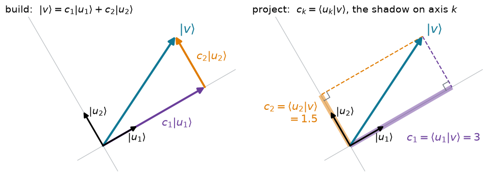

Fig. Left: the vector $\lvert v\rangle$ built from $c_1\lvert u_1\rangle$ and $c_2\lvert u_2\rangle$ , tip to tail. Right: the same coefficients found by projection; each $c_k = \langle u_k \vert v\rangle$ is the shadow of $\lvert v\rangle$ on its own axis. Here $c_1 = 3$ and $c_2 = 1.5$ .

A function: the same two steps¶

A wavefunction in a box is built the same way, with the box states $\lvert\psi_n\rangle$ , $\psi_n = \sqrt{2/L}\,\sin(n\pi x/L)$ , in place of the unit vectors. They are orthonormal, $\langle \psi_m \vert \psi_n\rangle = \delta_{mn}$ , and there are enough of them to build any state in the box:

\lvert\psi\rangle = c_1\lvert\psi_1\rangle + c_2\lvert\psi_2\rangle + c_3\lvert\psi_3\rangle + \cdots

(3)

The bra $\langle \psi_m\rvert$ picks out one coefficient, exactly as for the vector. The only new step is how to compute a bracket of two functions: multiply them point by point and integrate.

\langle \psi_m \vert \psi\rangle = \sum_n c_n\,\underbrace{\langle \psi_m \vert \psi_n\rangle}_{\delta_{mn}} = c_m, \qquad \langle \psi_m \vert \psi\rangle = \int_0^L \psi_m^*\,\psi\,dx

(4)

# synced: function_projection
import numpy as np
import matplotlib.pyplot as plt
from matplotlib.animation import FuncAnimation
from IPython.display import HTML

TEAL, CARDINAL, GRAY, PURPLE, ORANGE = "#107895", "#C8102E", "#6c757d", "#6a3d9a", "#e07b00"
plt.rcParams.update({"axes.spines.top": False, "axes.spines.right": False})
x = np.linspace(0, 1, 400)
psi = np.sqrt(30) * x * (1 - x)                             # the state of the worked example, L = 1
fig, axs = plt.subplots(1, 2, figsize=(9.6, 3.5), gridspec_kw={"wspace": 0.1})
for ax, n in zip(axs, (1, 2)):
    phi = np.sqrt(2) * np.sin(n * np.pi * x)
    prod = phi * psi
    c = np.trapezoid(prod, x)
    ax.fill_between(x, prod, where=prod >= 0, color=PURPLE, alpha=0.25, lw=0, interpolate=True)
    ax.fill_between(x, prod, where=prod < 0, color=ORANGE, alpha=0.3, lw=0, interpolate=True)
    ax.plot(x, psi, color=TEAL, lw=2.4, label=r"the state $\psi$")
    ax.plot(x, phi, color=GRAY, lw=1.6, ls="--", label=r"box state $\psi_n$")
    ax.plot(x, prod, color=PURPLE, lw=1.2, label=r"product $\psi_n\,\psi$")
    ax.axhline(0, color=GRAY, lw=0.6)
    ax.set_xlim(0, 1); ax.set_ylim(-1.75, 2.35); ax.set_yticks([])
    ax.set_xticks([0, 0.5, 1]); ax.set_xticklabels(["0", "L/2", "L"], fontsize=11)
    ax.spines["left"].set_visible(False)
    ax.set_title(rf"$c_1 = \langle\psi_1|\psi\rangle = \int\psi_1\,\psi\,dx = {abs(c):.3f}$" if n == 1
                 else r"$c_2 = \langle\psi_2|\psi\rangle = 0$: the lobes cancel", loc="left", fontsize=13)
axs[1].legend(loc="lower left", frameon=False, fontsize=11, handlelength=1.6, borderaxespad=0.1)
fig.subplots_adjust(left=0.01, right=0.99, top=0.88, bottom=0.1)
plt.show()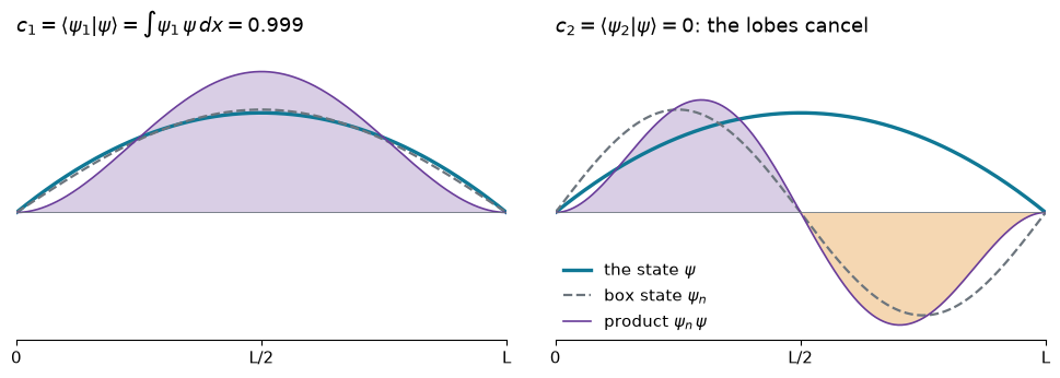

Fig. The state $\psi = \sqrt{30}\,x(1-x)$ in a box with $L = 1$ , projected onto the first two box states. Each coefficient $c_n = \langle \psi_n \vert \psi\rangle$ is the area under the product $\psi_n\psi$ : almost 1 for $n = 1$ , and exactly 0 for $n = 2$ , where the positive and negative lobes cancel.

Side by side, the vector and the function follow one structure. Only the last row, how a bracket is computed, differs:

	a vector in a plane	a function
axes	$\lvert u_1\rangle, \lvert u_2\rangle$	eigenfunctions $\lvert\phi_1\rangle, \lvert\phi_2\rangle, \dots$
orthonormal	$\langle u_j \vert u_k\rangle = \delta_{jk}$	$\langle \phi_m \vert \phi_n\rangle = \delta_{mn}$
build	$\lvert v\rangle = \sum_k c_k\lvert u_k\rangle$	$\lvert\psi\rangle = \sum_n c_n\lvert\phi_n\rangle$
project	$c_k = \langle u_k \vert v\rangle$	$c_n = \langle \phi_n \vert \psi\rangle$
the bracket	multiply matching components, add	multiply point by point, integrate

The box states are one set of axes. The eigenfunctions $\phi_n$ of any Hermitian operator are orthonormal and complete (Operators 2), so every state can be expanded in them:

Example: how much ground state is in a parabola?

The state $\psi = \sqrt{30/L^5}\;x(L-x)$ vanishes at both walls, so it is a legitimate particle-in-a-box state. Expand it in the box states $\psi_n = \sqrt{2/L}\,\sin(n\pi x/L)$ . Two integrations by parts give

c_n = \int_0^L \psi_n\,\psi\,dx = \frac{\sqrt{60}}{L^3}\int_0^L x(L-x)\sin\frac{n\pi x}{L}\,dx = \frac{\sqrt{60}}{L^3}\cdot\frac{2L^3\big[1-(-1)^n\big]}{(n\pi)^3}

(6)

c_n = \frac{8\sqrt{15}}{(n\pi)^3}\ \ (n \text{ odd}), \qquad c_n = 0\ \ (n \text{ even})

(7)

The even coefficients vanish by symmetry: the parabola is even about the center of the box and the even- $n$ states are odd. The first few probabilities are

\lvert c_1\rvert^2 = \frac{960}{\pi^6} = 0.9986, \qquad \lvert c_3\rvert^2 = \frac{960}{729\,\pi^6} = 0.0014, \qquad \lvert c_5\rvert^2 = 0.0001

(8)

The parabola is 99.86 percent ground state: the state and the box state in the left panel of the figure above are almost indistinguishable.

A smooth, spread-out state needs few eigenfunctions. A narrow one needs many, because it takes short wavelengths, high $n$ , to build a sharp feature:

# synced: sine_series
import numpy as np
import matplotlib.pyplot as plt
from matplotlib.animation import FuncAnimation
from IPython.display import HTML

TEAL, CARDINAL, GRAY, PURPLE, ORANGE = "#107895", "#C8102E", "#6c757d", "#6a3d9a", "#e07b00"
plt.rcParams.update({"axes.spines.top": False, "axes.spines.right": False})
x = np.linspace(0, 1, 600)
psi = np.exp(-(x - 0.3)**2 / (4 * 0.045**2))               # |psi|^2 has width 0.045 L
psi = psi / np.sqrt(np.trapezoid(psi**2, x))
ns = np.arange(1, 31)
phis = np.sqrt(2) * np.sin(np.outer(ns, np.pi * x))
c = np.trapezoid(phis * psi, x, axis=1)
ks = np.concatenate([np.arange(1, 25), np.full(6, 24)])
fig, (ax, axb) = plt.subplots(2, 1, figsize=(8, 4.4), gridspec_kw={"height_ratios": [1.5, 1], "hspace": 0.55})
ax.plot(x, psi, color="k", lw=1.4, ls=":", label=r"the state $\psi$")
(part,) = ax.plot([], [], color=TEAL, lw=2.4, label=r"sum of the first $k$ terms $c_n\psi_n$")
band = [ax.fill_between(x, 0 * x, color=TEAL, alpha=0.15, lw=0)]
ax.axhline(0, color=GRAY, lw=0.6)
ax.set_xlim(0, 1); ax.set_ylim(-1.6, 3.6); ax.set_yticks([])
ax.set_xticks([0, 0.5, 1]); ax.set_xticklabels(["0", "L/2", "L"], fontsize=12)
ax.spines["left"].set_visible(False)
ax.legend(loc="upper right", frameon=False, fontsize=12)
bars = axb.bar(ns, c**2, color="#d9dde1", width=0.75)
axb.set_xlim(0.3, 30.7); axb.set_ylim(0, 1.15 * (c**2).max())
axb.set_xlabel(r"$n$", fontsize=12); axb.set_ylabel(r"$|c_n|^2$", fontsize=12)
axb.set_yticks([0, 0.1]); axb.tick_params(labelsize=11)
fig.subplots_adjust(left=0.08, right=0.98, top=0.9, bottom=0.12)

def update(i):
    k = ks[i]
    s = c[:k] @ phis[:k]
    part.set_data(x, s)
    band[0].remove(); band[0] = ax.fill_between(x, s, color=TEAL, alpha=0.15, lw=0)
    for j, b in enumerate(bars):
        b.set_color(TEAL if j < k else "#d9dde1")
    ax.set_title(rf"$k = {k}$ box states", loc="left", fontsize=13)
    axb.set_title(f"the first {k} states hold probability {np.sum(c[:k]**2):.3f}", loc="left", fontsize=12.5)

ani = FuncAnimation(fig, update, frames=len(ks), interval=140, blit=False)
plt.close(fig)
HTML(ani.to_jshtml())

Fig. A narrow packet centered at $x = 0.3L$ rebuilt from box states one at a time. Top: the sum of the first $k$ terms $c_n\psi_n$ against the packet. Bottom: $\lvert c_n\rvert^2$ for each state, lit once it is included. About ten states are needed before the sum holds 99 percent of the probability.

A measurement returns an eigenvalue¶

The probabilities add up to one because the state is normalized. Expand both sides of $\langle \psi \vert \psi \rangle = 1$ ; orthonormality removes every cross term:

\langle \psi \vert \psi \rangle = \sum_m\sum_n c_m^*\,c_n\,\langle \phi_m \vert \phi_n \rangle = \sum_n \lvert c_n\rvert^2 = 1

(10)

Only the size of each coefficient matters for these probabilities. The coefficients $c_n$ and $c_n e^{i\theta}$ give the same $p_n$ ; the phases come back in Time Dependence.
A measurement does not reveal $\psi$ . It returns one number, and it changes the state (below). The probabilities show up only in the statistics of many identically prepared copies, just as $\lvert\psi(x)\rvert^2$ showed up in the pattern of many single detections in The Schrödinger Equation.

Try it: pick a state, measure one copy at a time, then a thousand. Every reading is one of the energies $E_n = n^2E_1$ of the box, never anything in between. The bars approach $\lvert c_n\rvert^2$ and the running mean approaches a value we compute next.

Averages and spreads¶

If the reading $a_n$ comes up with probability $p_n$ , the average over many readings is the weighted sum $\sum_n p_n a_n$ . The integral formula of The Schrödinger Equation gives the same number. Expand $\psi$ and let $\hat{A}$ act on each eigenfunction:

\langle \psi \vert \hat{A} \vert \psi \rangle = \sum_m\sum_n c_m^*\,c_n\,\langle \phi_m \vert \hat{A} \vert \phi_n \rangle = \sum_m\sum_n c_m^*\,c_n\,a_n\,\delta_{mn} = \sum_n \lvert c_n\rvert^2\,a_n

(11)

The spread is a sum of squares weighted by probabilities, so it vanishes only when all the probability sits on one eigenvalue: only an eigenfunction gives a sharp value.

Example: energy readings of a superposition

A particle in a box is in the state $\psi = \tfrac{1}{2}\psi_1 + \tfrac{1}{2}\psi_2 + \tfrac{1}{\sqrt{2}}\psi_3$ , the default state of the widget. What readings are possible, how often, and what are their average and spread?

The readings are $E_1$ , $4E_1$ and $9E_1$ , with probabilities $\tfrac{1}{4}$ , $\tfrac{1}{4}$ and $\tfrac{1}{2}$ , which add up to one. Then

\langle E \rangle = \tfrac{1}{4}E_1 + \tfrac{1}{4}\cdot4E_1 + \tfrac{1}{2}\cdot9E_1 = \tfrac{23}{4}E_1 = 5.75\,E_1

(14)

\langle E^2 \rangle = \tfrac{1}{4}E_1^2 + \tfrac{1}{4}\cdot16E_1^2 + \tfrac{1}{2}\cdot81E_1^2 = 44.75\,E_1^2, \qquad \sigma_E = \sqrt{44.75 - 5.75^2}\;E_1 = 3.42\,E_1

(15)

The average, $5.75\,E_1$ , is not one of the possible readings. No single measurement ever returns it.

The two routes to $\langle E \rangle$ , the sum over probabilities and the integral, are worth checking numerically. On a grid the box states are the eigenvectors of the Hamiltonian matrix, and the expansion coefficients are dot products:

import numpy as np

N = 1000                                          # interior points of a box with L = 1
x = np.linspace(0, 1, N + 2)[1:-1]; dx = x[1] - x[0]
H = (2 * np.eye(N) - np.eye(N, k=1) - np.eye(N, k=-1)) / (2 * dx**2)   # hbar = m = 1, V = 0
E, phi = np.linalg.eigh(H)
phi = phi / np.sqrt(dx)                           # columns normalized as functions
E1 = np.pi**2 / 2                                 # exact ground-state energy

psi = np.sqrt(30) * x * (1 - x)                   # the parabola of the example
c = phi.T @ psi * dx                              # c_n = <phi_n|psi>
p = c**2

print("p_1, p_2, p_3:", np.round(p[:3], 5))
print("sum of p_n:", round(p.sum(), 6))
print("<E> = sum p_n E_n:", round(p @ E / E1, 4), "E1")
print("<E> = <psi|H|psi>:", round(psi @ H @ psi * dx / E1, 4), "E1   (exact: 10/pi^2 =", round(10 / np.pi**2, 4), "E1)")

p_1, p_2, p_3: [0.99856 0.      0.00137]
sum of p_n: 1.0
<E> = sum p_n E_n: 1.0132 E1
<E> = <psi|H|psi>: 1.0132 E1   (exact: 10/pi^2 = 1.0132 E1)

The grid agrees with the exact coefficients of the example, and both routes give $\langle E \rangle = 10E_1/\pi^2 = 1.013\,E_1$ : the parabola costs only 1.3 percent more energy than the ground state.
The translation table of Operators 1 grows by the three rows this lecture used:

	integral	Dirac	numpy on a grid
expansion coefficient	$c_n = \int \phi_n^*\,\psi\,dx$	$c_n = \langle \phi_n \vert \psi \rangle$	`c = phi.conj().T @ psi * dx`
probability of $a_n$	$\lvert c_n\rvert^2$	$\lvert\langle \phi_n \vert \psi \rangle\rvert^2$	`p = np.abs(c)**2`
average	$\sum_n \lvert c_n\rvert^2 a_n$	$\langle \psi \vert \hat{A} \vert \psi \rangle$	`p @ a`

After the measurement¶

# synced: collapse
import numpy as np
import matplotlib.pyplot as plt
from matplotlib.animation import FuncAnimation
from IPython.display import HTML

TEAL, CARDINAL, GRAY, PURPLE, ORANGE = "#107895", "#C8102E", "#6c757d", "#6a3d9a", "#e07b00"
plt.rcParams.update({"axes.spines.top": False, "axes.spines.right": False})
x = np.linspace(0, 1, 400)
ph = [np.sqrt(2) * np.sin(n * np.pi * x) for n in (1, 2, 3, 4)]
before = np.array([0.5, 0.5, np.sqrt(0.5), 0])
after = np.array([0, 0, 1.0, 0])
fig = plt.figure(figsize=(8.6, 3.9))
gs = fig.add_gridspec(2, 3, width_ratios=[1, 0.42, 1], height_ratios=[1.1, 1], hspace=0.35, wspace=0.05)
for col, cs, title in ((0, before, r"before: $\psi = \frac{1}{2}\psi_1 + \frac{1}{2}\psi_2 + \frac{1}{\sqrt{2}}\psi_3$"),
                       (2, after, r"after: $\psi = \psi_3$")):
    ax, axb = fig.add_subplot(gs[0, col]), fig.add_subplot(gs[1, col])
    w = sum(ci * p for ci, p in zip(cs, ph))
    ax.fill_between(x, w**2, color=CARDINAL, alpha=0.15, lw=0)
    ax.plot(x, w, color=TEAL, lw=2.4); ax.plot(x, w**2, color=CARDINAL, lw=1.6)
    ax.axhline(0, color=GRAY, lw=0.6); ax.set_xlim(0, 1); ax.set_ylim(-2.2, 4.3)
    ax.set_xticks([]); ax.set_yticks([]); ax.spines["left"].set_visible(False); ax.spines["bottom"].set_visible(False)
    ax.set_title(title, loc="left", fontsize=12)
    axb.bar([1, 2, 3, 4], cs**2, color=TEAL, width=0.6)
    axb.set_xticks([1, 2, 3, 4]); axb.set_xticklabels([r"$E_1$", r"$4E_1$", r"$9E_1$", r"$16E_1$"], fontsize=12)
    axb.set_ylim(0, 1.08); axb.set_yticks([0, 0.5, 1]); axb.tick_params(axis="y", labelsize=10.5)
    if col == 0:
        axb.set_ylabel("probability", fontsize=11)
    else:
        axb.set_yticklabels([])
axm = fig.add_subplot(gs[:, 1]); axm.axis("off")
axm.annotate("", xy=(0.95, 0.55), xytext=(0.05, 0.55), xycoords="axes fraction",
             arrowprops=dict(arrowstyle="simple,head_length=0.9,head_width=0.9,tail_width=0.35", color=PURPLE, alpha=0.8))
axm.text(0.5, 0.68, "measure $E$", ha="center", fontsize=12.5, color=PURPLE)
axm.text(0.5, 0.49, "reading: $9E_1$", ha="center", va="top", fontsize=12.5, color=PURPLE)
fig.text(0.5, 0.01, r"measuring again right away gives $9E_1$ every time; a fresh copy of the old state gives $E_1$, $4E_1$ or $9E_1$",
         ha="center", fontsize=11.5, color=GRAY)
fig.subplots_adjust(left=0.06, right=0.99, top=0.9, bottom=0.14)
plt.show()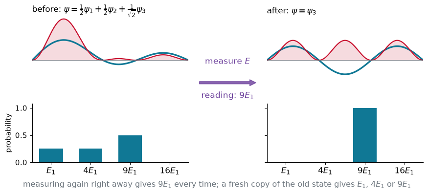

Fig. One energy measurement on the superposition of the example. Before: three possible readings, with probabilities $\frac{1}{4}$ , $\frac{1}{4}$ and $\frac{1}{2}$ . The reading happens to be $9E_1$ . After: the state is $\psi_3$ , and all the probability sits on $9E_1$ .

Orthogonal eigenfunctions are mutually exclusive outcomes: a system found in $\phi_1$ has zero overlap with $\phi_2$ . A single copy never returns a mixture of readings; the mixture lives in the statistics of many copies.
What happens physically during the collapse is the oldest open question of quantum mechanics. The Copenhagen interpretation, worked out by Bohr and Heisenberg in the 1920s and the one most often taught, holds that a system has no definite value of $A$ before it is measured; the theory predicts only the probabilities, and the measurement produces one outcome. Schrödinger found this absurd and made his point with a cat:

Compatible and incompatible observables¶

If $[\hat{A},\hat{B}] = 0$ , the two operators share eigenfunctions (Operators 2). A reading of $a_n$ leaves the system in a shared eigenfunction, so $B$ is sharp too, and measuring $B$ does not disturb the value of $A$ . Such observables are compatible: energy and momentum of a free particle, or $\hat{H}$ , $\hat{L}^2$ and $\hat{L}_z$ for hydrogen.
If they do not commute, a state with a sharp value of one has a spread in the other. The box states have sharp energies; their momenta are not sharp:

# synced: box_momentum
import numpy as np
import matplotlib.pyplot as plt
from matplotlib.animation import FuncAnimation
from IPython.display import HTML

TEAL, CARDINAL, GRAY, PURPLE, ORANGE = "#107895", "#C8102E", "#6c757d", "#6a3d9a", "#e07b00"
plt.rcParams.update({"axes.spines.top": False, "axes.spines.right": False})
x = np.linspace(0, 1, 2000)                                 # L = hbar = 1: p in units of pi hbar / L
p = np.linspace(-8, 8, 800)
kern = np.exp(-1j * np.outer(p * np.pi, x)) / np.sqrt(2 * np.pi)
fig, axs = plt.subplots(3, 1, figsize=(8, 4.6), sharex=True, gridspec_kw={"hspace": 0.45})
for ax, n, col in zip(axs, (1, 2, 5), (TEAL, PURPLE, CARDINAL)):
    amp = np.trapezoid(kern * np.sqrt(2) * np.sin(n * np.pi * x), x, axis=1)
    dens = np.abs(amp)**2 * np.pi                           # density per unit of p / (pi hbar / L)
    ax.fill_between(p, dens, color=col, alpha=0.2, lw=0); ax.plot(p, dens, color=col, lw=2.2)
    for s in (-n, n):
        ax.axvline(s, color=GRAY, lw=1, ls="--")
    ax.set_yticks([]); ax.spines["left"].set_visible(False)
    ax.set_ylim(0, 1.15 * dens.max())
    ax.set_title(rf"$n = {n}$:  dashed lines at $p = \pm\sqrt{{2mE_{n}}} = \pm {n}\,\pi\hbar/L$", loc="left", fontsize=12)
axs[-1].set_xlabel(r"momentum $p$  (units of $\pi\hbar/L$)", fontsize=12)
axs[-1].tick_params(labelsize=11)
fig.subplots_adjust(left=0.03, right=0.98, top=0.93, bottom=0.12)
plt.show()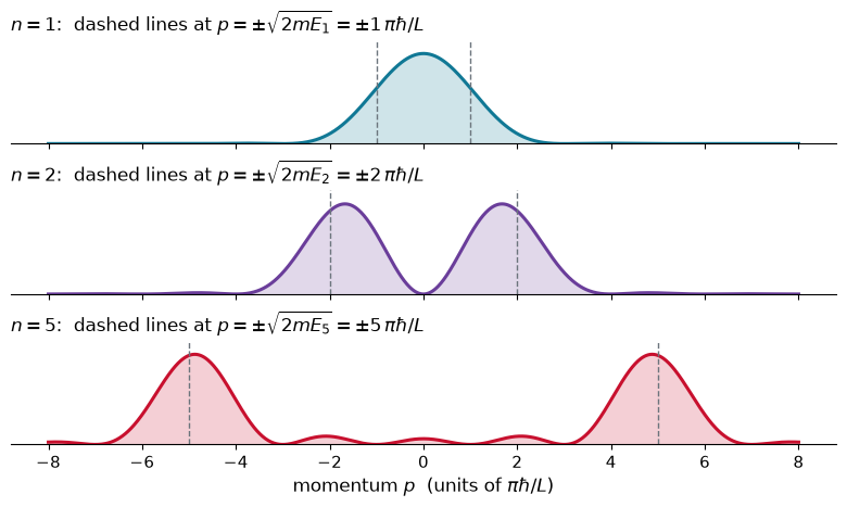

Fig. Momentum distributions of three particle-in-a-box states. The sine is half a wave moving right and half moving left, $\sin kx = (e^{ikx} - e^{-ikx})/2i$ , so the distribution has humps near $p = \pm n\pi\hbar/L = \pm\sqrt{2mE_n}$ . The walls cut the wave off after a length $L$ , which broadens each hump by about $h/L$ . For $n = 1$ the two humps merge into one.

How much spread the commutator forces is the uncertainty principle, the general form of the relation met in Chapter 1:

For position and momentum the commutator is the constant $i\hbar$ , so its average is $i\hbar$ in every state, and the bound $\hbar/2$ is the same for every state. Squeezing the position spread widens the momentum spread:

# synced: uncertainty_tradeoff
import numpy as np
import matplotlib.pyplot as plt
from matplotlib.animation import FuncAnimation
from IPython.display import HTML

TEAL, CARDINAL, GRAY, PURPLE, ORANGE = "#107895", "#C8102E", "#6c757d", "#6a3d9a", "#e07b00"
plt.rcParams.update({"axes.spines.top": False, "axes.spines.right": False})
nf = 40
sx = np.exp(np.log(1.4) + (np.log(0.3) - np.log(1.4)) * 0.5 * (1 - np.cos(2 * np.pi * np.arange(nf) / nf)))
x = np.linspace(-4, 4, 500)                                 # hbar = 1
fig = plt.figure(figsize=(9, 3.4))
gs = fig.add_gridspec(1, 3, width_ratios=[1, 1, 1.05], wspace=0.35)
axx, axp, axu = (fig.add_subplot(gs[0, j]) for j in range(3))
(lx,) = axx.plot([], [], color=TEAL, lw=2.4); bx = [axx.fill_between(x, 0 * x, color=TEAL, alpha=0.2, lw=0)]
(lp,) = axp.plot([], [], color=CARDINAL, lw=2.4); bp = [axp.fill_between(x, 0 * x, color=CARDINAL, alpha=0.2, lw=0)]
for ax, lab in ((axx, r"position $x$"), (axp, r"momentum $p$")):
    ax.set_xlim(-4, 4); ax.set_ylim(0, 1.45); ax.set_yticks([]); ax.spines["left"].set_visible(False)
    ax.set_xlabel(lab, fontsize=12); ax.tick_params(labelsize=10.5)
dx = np.geomspace(0.08, 3, 200)
axu.fill_between(dx, 0.04, 0.5 / dx, color=GRAY, alpha=0.25, lw=0)
axu.plot(dx, 0.5 / dx, color="k", lw=1.6)
axu.plot(dx, 0.568 / dx, color=PURPLE, lw=1.4, ls="--")
axu.text(0.1, 0.35, "forbidden:\n" + r"$\Delta x\,\Delta p < \hbar/2$", fontsize=11, color=GRAY, va="bottom")
(gdot,) = axu.plot([], [], "o", color=TEAL, ms=10, zorder=5, label=r"Gaussian: $\Delta x\Delta p = 0.50\,\hbar$")
(bdot,) = axu.plot([], [], "s", color=PURPLE, ms=9, zorder=5, label=r"box ground state: $0.57\,\hbar$")
axu.set_xscale("log"); axu.set_yscale("log"); axu.set_xlim(0.08, 3); axu.set_ylim(0.04, 12)
axu.set_xlabel(r"$\Delta x$", fontsize=12); axu.set_ylabel(r"$\Delta p$", fontsize=12); axu.tick_params(labelsize=10)
axu.legend(loc="upper right", frameon=False, fontsize=10.5, handletextpad=0.3, borderaxespad=0.1)
fig.subplots_adjust(left=0.02, right=0.98, top=0.86, bottom=0.17)

def update(i):
    s = sx[i]; sp = 0.5 / s
    rx = np.exp(-x**2 / (2 * s**2)) / np.sqrt(2 * np.pi * s**2)
    rp = np.exp(-x**2 / (2 * sp**2)) / np.sqrt(2 * np.pi * sp**2)
    lx.set_data(x, rx); bx[0].remove(); bx[0] = axx.fill_between(x, rx, color=TEAL, alpha=0.2, lw=0)
    lp.set_data(x, rp); bp[0].remove(); bp[0] = axp.fill_between(x, rp, color=CARDINAL, alpha=0.2, lw=0)
    axx.set_title(rf"$|\psi(x)|^2$:  $\Delta x = {s:.2f}$", loc="left", fontsize=12.5)
    axp.set_title(rf"$|\phi(p)|^2$:  $\Delta p = {sp:.2f}$", loc="left", fontsize=12.5)
    gdot.set_data([s], [sp]); bdot.set_data([s], [0.568 / s])
    axu.set_title(rf"$\Delta x\,\Delta p = {s * sp:.2f}\,\hbar$", loc="left", fontsize=12.5)

ani = FuncAnimation(fig, update, frames=nf, interval=120, blit=False)
plt.close(fig)
HTML(ani.to_jshtml())

Fig. A Gaussian squeezed and released. Left: the position distribution. Middle: the momentum distribution, which widens as the position narrows. Right: the two spreads on log axes. The gray region below $\sigma_x\sigma_p = \hbar/2$ is forbidden. The Gaussian rides exactly on the boundary, the least uncertain state possible; the ground state of a box of matching size (square) sits a little above it, at $0.57\,\hbar$ .

Example: how uncertain is the box ground state?

For $\psi_1 = \sqrt{2/L}\,\sin(\pi x/L)$ : the average position is $L/2$ by symmetry, and $\langle x^2\rangle = L^2\big(\tfrac{1}{3} - \tfrac{1}{2\pi^2}\big)$ , so

\sigma_x = L\sqrt{\frac{1}{12} - \frac{1}{2\pi^2}} = 0.181\,L

(17)

The average momentum is zero, and $\langle p^2\rangle = 2mE_1 = (\pi\hbar/L)^2$ , so $\sigma_p = \pi\hbar/L$ . The product

\sigma_x\,\sigma_p = 0.181\,\pi\,\hbar = 0.568\,\hbar \geq 0.5\,\hbar

(18)

does not depend on $L$ : a smaller box localizes the particle better and raises its momentum spread by the same factor. This is also why confinement costs energy. Squeezing the box raises $\sigma_p$ , and the kinetic energy $\langle p^2\rangle/2m$ grows as $1/L^2$ .

Problems¶

Problem 1: Complex coefficients¶

A particle in a box is in the state $\psi = \frac{1}{\sqrt{2}}\big(\psi_1 + i\,\psi_2\big)$ . What energies can be measured, with what probabilities? Find $\langle E\rangle$ and $\sigma_E$ .

Solution

The probabilities are the squared magnitudes, $\lvert 1/\sqrt{2}\rvert^2 = \lvert i/\sqrt{2}\rvert^2 = \tfrac{1}{2}$ : half the readings give $E_1$ , half give $4E_1$ . The factor $i$ does not change them. Then

\langle E\rangle = \tfrac{1}{2}E_1 + \tfrac{1}{2}\cdot4E_1 = 2.5\,E_1, \qquad \langle E^2\rangle = \tfrac{1}{2}E_1^2 + \tfrac{1}{2}\cdot16E_1^2 = 8.5\,E_1^2

(19)

\sigma_E = \sqrt{8.5 - 6.25}\;E_1 = 1.5\,E_1

(20)

The $i$ is not invisible to every measurement. It changes where the particle is likely to be found (compare Problem 8), and it changes how the state moves in time.

Problem 2: Averages of observables are real¶

Show that $\langle A\rangle = \langle \psi \vert \hat{A} \vert \psi \rangle$ is a real number whenever $\hat{A}$ is Hermitian, for every state $\psi$ .

Solution

Take the complex conjugate and use $\langle f \vert g\rangle^* = \langle g \vert f\rangle$ , then the Hermitian property:

\langle A\rangle^* = \langle \psi \vert \hat{A}\psi \rangle^* = \langle \hat{A}\psi \vert \psi \rangle = \langle \psi \vert \hat{A}\psi \rangle = \langle A\rangle

(21)

A number equal to its own conjugate is real. The expansion gives the same conclusion: $\langle A\rangle = \sum_n p_n a_n$ is a sum of real eigenvalues with positive weights.

Problem 3: Two measurements in a row¶

A particle in a box is in the state $\psi = \frac{1}{2}\big(\sqrt{3}\,\psi_1 + \psi_2\big)$ . (a) What is the probability that an energy measurement gives $E_1$ ? (b) The reading is in fact $4E_1$ . What is the state right after, and what does a second energy measurement give? (c) Next the position is measured. Where is the particle never found?

Solution

(a) $\lvert\sqrt{3}/2\rvert^2 = \tfrac{3}{4}$ .

(b) The reading $4E_1$ leaves the particle in $\psi_2$ . A second energy measurement returns $4E_1$ with probability one: $\psi_2$ is an eigenfunction of $\hat{H}$ .

(c) The position distribution is now $\lvert\psi_2(x)\rvert^2 = \frac{2}{L}\sin^2(2\pi x/L)$ , which vanishes at the node $x = L/2$ (and at the walls). Before the energy measurement the distribution was $\lvert\psi\rvert^2$ , which does not vanish at the center: the first measurement changed what the second one sees.

Problem 4: The spread of the parabola¶

For the parabola $\psi = \sqrt{30/L^5}\,x(L-x)$ of the worked example, 99.86 percent of the energy readings give exactly $E_1$ . Find $\sigma_E$ , using $\sum_{n\ \text{odd}} 1/n^2 = \pi^2/8$ and $\sum_{n\ \text{odd}} 1/n^4 = \pi^4/96$ .

Solution

With $p_n = 960/(n\pi)^6$ for odd $n$ and $E_n = n^2E_1$ :

\langle E\rangle = \sum_{n\ \text{odd}} \frac{960}{\pi^6 n^6}\,n^2E_1 = \frac{960}{\pi^6}\cdot\frac{\pi^4}{96}\,E_1 = \frac{10}{\pi^2}E_1, \qquad \langle E^2\rangle = \frac{960}{\pi^6}\sum_{n\ \text{odd}}\frac{1}{n^2}\,E_1^2 = \frac{120}{\pi^4}E_1^2

(22)

\sigma_E = \sqrt{\frac{120}{\pi^4} - \frac{100}{\pi^4}}\;E_1 = \frac{\sqrt{20}}{\pi^2}\,E_1 = 0.45\,E_1

(23)

The spread is large although almost every reading is $E_1$ , because the rare readings are far away: $9E_1$ , $25E_1$ , and so on. A standard deviation weights distant outliers heavily.

Problem 5: Expanding a tent¶

The tent state rises linearly from zero at $x = 0$ to a peak at $x = L/2$ and falls back linearly to zero at $x = L$ . Normalize it, then find its expansion coefficients in box states, either by integrating by parts or numerically with the grid code above. What is the probability of measuring $E_1$ ? How many states hold 99.9 percent of the probability? Compare with the parabola, and explain the difference using the sharp corner of the tent.

Problem 6: Momentum of the ground state¶

Compute the momentum distribution $\lvert\phi_1(p)\rvert^2$ of the box ground state numerically, from $\phi_1(p) = (2\pi\hbar)^{-1/2}\int_0^L \psi_1(x)\,e^{-ipx/\hbar}\,dx$ . Check that it is normalized and that its spread is $\sigma_p = \pi\hbar/L$ . Why is it largest at $p = 0$ rather than at $p = \pm\pi\hbar/L$ ?

Problem 7: An uncertainty relation for energy and position¶

Use $[\hat{x},\hat{H}] = i\hbar\,\hat{p}/m$ (Problem 5 of Operators 2 leads to it) in the general uncertainty principle to show $\sigma_x\,\sigma_E \geq \frac{\hbar}{2m}\lvert\langle p\rangle\rvert$ . Evaluate the bound for a box eigenstate and for a free packet moving with average momentum $p_0$ . Why does a stationary state escape any constraint?

Problem 8: Phases you can see¶

The states $\psi_\pm = \frac{1}{\sqrt{2}}\big(\psi_1 \pm \psi_2\big)$ in a box give identical energy statistics. Compute $\langle x\rangle$ for each, and sketch $\lvert\psi_\pm\rvert^2$ . Which measurement tells them apart, and why can no energy measurement do it?