Operators 1: Matrices and Dirac Notation

What you need to know

An operator turns one function into another. Quantum operators are linear, so they respect superposition: acting on a sum gives the sum of the results.
A matrix is the linear operator you already know: it turns and stretches arrows. The arrows it only stretches are its eigenvectors, $A\mathbf{v} = \lambda\mathbf{v}$ , and for a $2\times 2$ matrix the eigenvalues come from a quadratic equation.
Sample a function on a grid and it becomes a vector; every operator becomes a matrix. Position is diagonal, derivatives link neighboring points, and solving $\hat{H}\psi = E\psi$ becomes finding the eigenvalues of a matrix: by hand for three points, with five lines of numpy for four hundred.
Dirac notation writes the same objects once. A ket is a column, a bra is the conjugated row, a bra meeting a ket is an inner product, and a bra, an operator and a ket together give a matrix element. Every line translates into an integral and into numpy.
The entries of a matrix depend on the axes you write it in. In the axes of its own eigenvectors a matrix is diagonal, with the eigenvalues on the diagonal, and finding those axes is what diagonalizing a Hamiltonian means.
Two matrix properties matter next: some matrices equal their own mirror image (Hermitian), and the order of a product can matter (commutators). Both are the subject of Operators 2.

The rules of the game¶

This lecture and the next three complete the short list of rules, the postulates, from which all of quantum mechanics follows. Two of them we have already met.

	Postulate	Lecture
1	The state of a system is a wavefunction $\psi$ , and $\lvert\psi\rvert^2$ is the probability density	The Schrödinger Equation
2	Every observable is represented by a linear Hermitian operator $\hat{A}$	this lecture and Operators 2
3	A measurement of $A$ returns one of the eigenvalues $a_n$ of $\hat{A}$ and leaves the system in its eigenfunction $\phi_n$	Measurement
4	The outcome $a_n$ has probability $\lvert\langle \phi_n \vert \psi\rangle\rvert^2$ , so the average is $\langle A\rangle = \langle \psi \vert \hat{A} \vert \psi \rangle$	Measurement
5	The state evolves by $i\hbar\,\partial\Psi/\partial t = \hat{H}\Psi$	The Schrödinger Equation, Time Dependence

Operators act on functions¶

In The Schrödinger Equation we built operators by a recipe: write the classical expression in $x$ and $p$ , then replace $p$ by $-i\hbar\,d/dx$ . We also met eigenfunctions, the functions an operator returns unchanged up to a constant, and expectation values.
The recipe leaves two questions open: which operators are allowed to stand for something we can measure, and what happens when two operators do not commute? Operators 2 answers both. This lecture builds the language they need: functions become vectors, and operators become matrices.
An operator is any rule that turns a function into another function: multiply by $x$ , differentiate, integrate, square. Quantum mechanics uses only one kind.

Linear operators¶

Linearity is what superposition demands. If $\Psi_1$ and $\Psi_2$ both solve $i\hbar\,\partial\Psi/\partial t = \hat{H}\Psi$ , their sum is again a solution only when $\hat{H}$ is linear. Interference, from the double slit to the sloshing particle in a box, shows that sums of states are states, so the operators must be linear.
Derivatives and multiplication by a function are linear: the derivative of a sum is the sum of the derivatives. Squaring, square roots and logarithms are not.

Example: two tests for linearity

Is the kinetic energy operator $\hat{K} = -\frac{\hbar^2}{2m}\frac{d^2}{dx^2}$ linear? Is squaring, $\hat{S}f = f^2$ ?

\hat{K}\big(c_1f_1 + c_2f_2\big) = -\frac{\hbar^2}{2m}\big(c_1f_1'' + c_2f_2''\big) = c_1\hat{K}f_1 + c_2\hat{K}f_2

(2)

so $\hat{K}$ is linear. For squaring,

\hat{S}\big(c_1f_1 + c_2f_2\big) = c_1^2f_1^2 + 2c_1c_2f_1f_2 + c_2^2f_2^2 \ne c_1f_1^2 + c_2f_2^2

(3)

The squared constants and the cross term $2c_1c_2f_1f_2$ both spoil it. A quick first test: a linear operator must turn $2f$ into $2\hat{A}f$ , and squaring turns it into $4f^2$ .

Matrices act on vectors¶

The linear operators you already know are matrices. Before turning functions into vectors, here is what a matrix does to an ordinary arrow in the plane. Vectors and Linear Algebra in Appendix A has more.

A matrix acts on a vector row by column: each entry of the result is one row of the matrix times the column, entry by entry, added up. For $A = \begin{pmatrix} 2 & 1 \\ 1 & 2 \end{pmatrix}$ ,

A\begin{pmatrix} 1 \\ 0 \end{pmatrix} = \begin{pmatrix} 2\cdot 1 + 1\cdot 0 \\ 1\cdot 1 + 2\cdot 0 \end{pmatrix} = \begin{pmatrix} 2 \\ 1 \end{pmatrix}, \qquad A\begin{pmatrix} 1 \\ 1 \end{pmatrix} = \begin{pmatrix} 3 \\ 3 \end{pmatrix} = 3\begin{pmatrix} 1 \\ 1 \end{pmatrix}

(4)

The first arrow is turned as well as stretched. The second keeps its direction and is only stretched, by a factor of 3.

Fig. The matrix $A$ turns a generic arrow (left) but only stretches its eigenvectors (right): $(1, 1)$ by a factor 3 and $(1, -1)$ by a factor 1.

Try it: drag anywhere on the plane to aim the unit arrow $\mathbf{v}$ and watch $A\mathbf{v}$ . Most directions come out turned. Hunt for the two directions that are only stretched; the widget marks each one you find. Sweep carries $\mathbf{v}$ once around the circle, pausing on each eigenvector, while the tips of $A\mathbf{v}$ trace an ellipse.

This has the same shape as the eigenvalue equation $\hat{A}\phi = a\phi$ of The Schrödinger Equation, with a matrix in place of the operator and a vector in place of the function.
Why the determinant? $(A - \lambda I)\mathbf{v} = 0$ says that the matrix $A - \lambda I$ squashes the nonzero arrow $\mathbf{v}$ to zero. A matrix that squashes some arrow to zero flattens the plane, so the area factor it multiplies areas by, its determinant, is zero. For a $2\times 2$ matrix the condition is a quadratic equation:

\det\begin{pmatrix} a - \lambda & b \\ c & d - \lambda \end{pmatrix} = (a - \lambda)(d - \lambda) - bc = \lambda^2 - (a + d)\,\lambda + (ad - bc) = 0

(6)

The roots of $\lambda^2 - s\lambda + p = 0$ add up to $s$ and multiply to $p$ . So the eigenvalues of a $2\times 2$ matrix add up to $a + d$ , the sum of its diagonal entries, called the trace, and multiply to $ad - bc$ , the determinant. These two numbers give a quick check on any eigenvalue calculation.

Example: eigenvalues of a $2\times 2$ by hand

Find the eigenvalues and eigenvectors of $A = \begin{pmatrix} 2 & 1 \\ 1 & 2 \end{pmatrix}$ .

\det(A - \lambda I) = (2 - \lambda)^2 - 1 = 0 \quad\Longrightarrow\quad 2 - \lambda = \pm 1 \quad\Longrightarrow\quad \lambda = 3,\ 1

(7)

For $\lambda = 3$ , the first row of $(A - 3I)\mathbf{v} = 0$ reads $-v_1 + v_2 = 0$ , so $\mathbf{v} \propto (1, 1)$ . For $\lambda = 1$ it reads $v_1 + v_2 = 0$ , so $\mathbf{v} \propto (1, -1)$ . Two quick checks: the eigenvalues add up to the trace, $3 + 1 = 2 + 2$ , and multiply to the determinant, $3 \times 1 = 2\cdot 2 - 1\cdot 1$ .

From operators to matrices¶

A computer cannot store a function, only a list of numbers. Turning functions into lists and operators into tables of numbers is how every quantum chemistry program works, and it makes the abstract properties of operators, Hermitian or commuting, concrete enough to check by eye. We build the dictionary in four steps. Operators as Matrices in Appendix A has more on each.

# synced: grid_roadmap
import numpy as np
import matplotlib.pyplot as plt
from matplotlib.animation import FuncAnimation
from IPython.display import HTML

TEAL, CARDINAL, GRAY, PURPLE, ORANGE = "#107895", "#C8102E", "#6c757d", "#6a3d9a", "#e07b00"
from matplotlib.patches import Rectangle, FancyBboxPatch
plt.rcParams.update({"axes.spines.top": False, "axes.spines.right": False})
W, Ht = 9.6, 3.75                                           # draw in inches: one data unit = one inch
fig = plt.figure(figsize=(W, Ht))
ax = fig.add_axes([0, 0, 1, 1]); ax.set_xlim(0, W); ax.set_ylim(0, Ht); ax.axis("off")
look = {"": ("white", "#ced4da", 1), "C": ("#fbeaec", CARDINAL, 2), "P": ("#f1ecf7", PURPLE, 2), "O": ("#fdf0e0", ORANGE, 2)}
s, n = 0.16, 5                                              # icon cell size and matrix size
xs, ytop, yic = [1.45, 3.3, 5.15, 7.0], 2.95, 1.2           # step columns, calculus row, grid row

def block(xc, rows, cols, kind):                            # rows x cols cells centred on (xc, yic); kind(r, c) picks the colour
    for r in range(rows):
        for c in range(cols):
            fc, ec, z = look[kind(r, c)]
            ax.add_patch(Rectangle((xc + (c - cols / 2) * s, yic + (rows / 2 - 1 - r) * s), s, s, fc=fc, ec=ec, lw=1, zorder=z))

tops = [r"$\psi(x)$", r"$x,\ \ V(x)$", r"$\dfrac{d}{dx},\ \ \dfrac{d^2}{dx^2}$", r"$\hat{H}\psi = E\,\psi$"]
verbs = ["sample", "multiply\npoint by point", "compare\nneighbors", "assemble"]
lows = [r"column of samples $\psi_j$", "diagonal matrix", "rows that link\nneighbors: $D_1$, $D_2$",
        "matrix $H$:\n$H\\mathbf{v} = E\\mathbf{v}$"]
kinds = [None, lambda r, c: "P" if r == c else "", lambda r, c: "O" if abs(r - c) <= 1 else "",
         lambda r, c: "P" if r == c else ("O" if abs(r - c) == 1 else "")]
ax.plot([0.55, W - 0.1], [2.4, 2.4], color=GRAY, lw=0.8, ls=(0, (4, 4)), alpha=0.6)
ax.text(0.3, ytop, "calculus", rotation=90, ha="center", va="center", fontsize=13, color=TEAL, style="italic")
ax.text(0.3, yic, "on a grid", rotation=90, ha="center", va="center", fontsize=13, color=CARDINAL, style="italic")
for k, (x, top, verb, low, kind) in enumerate(zip(xs, tops, verbs, lows, kinds), start=1):
    ax.text(x, ytop + 0.5, f"Step {k}", ha="center", va="center", fontsize=12.5, color=GRAY)
    ax.add_patch(FancyBboxPatch((x - 0.75, ytop - 0.31), 1.5, 0.62, boxstyle="round,pad=0,rounding_size=0.12",
                                fc="#e3f1f5", ec=TEAL, lw=1.4))
    ax.text(x, ytop, top, ha="center", va="center", fontsize=15)
    ax.annotate("", xy=(x, yic + 0.52), xytext=(x, ytop - 0.36),
                arrowprops=dict(arrowstyle="-|>", color=GRAY, lw=1.6, mutation_scale=16, shrinkA=0, shrinkB=0))
    ax.text(x + 0.1, 2.03, verb, ha="left", va="center", fontsize=12, color=GRAY, linespacing=1.15)
    if kind is None:
        block(x, n, 1, lambda r, c: "C")
    else:
        block(x, n, n, kind)
    ax.text(x, yic - n * s / 2 - 0.13, low, ha="center", va="top", fontsize=12.5, linespacing=1.25)
xr = 8.75                                                   # the payoff: eigh turns H into energies and states
ax.annotate("", xy=(xr - 0.42, yic), xytext=(xs[3] + n * s / 2 + 0.12, yic),
            arrowprops=dict(arrowstyle="-|>", color=GRAY, lw=1.6, mutation_scale=16, shrinkA=0, shrinkB=0))
ax.text((xr - 0.42 + xs[3] + n * s / 2 + 0.12) / 2, yic + 0.12, "eigh", ha="center", va="bottom", fontsize=13.5,
        family="monospace", color="k")
for k in range(4):
    ax.plot([xr - 0.3, xr + 0.3], [yic - 0.36 + 0.24 * k] * 2, color="k", lw=2.4, solid_capstyle="butt")
ax.text(xr, yic - n * s / 2 - 0.13, "energies $E_n$,\nstates $\\mathbf{v}_n$", ha="center", va="top", fontsize=12.5,
        linespacing=1.25)
plt.show()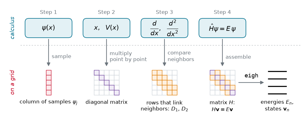

Fig. The four steps of this section. Each one trades something from calculus (top row) for something a computer can store (bottom row): the function for a column of samples, multiplication for a diagonal matrix, derivatives for rows that link neighbors, and the Schrödinger equation for a matrix whose eigenvalues eigh finds.

Step 1: a function becomes a vector¶

A vector is a list of numbers, its components. The arrow $(2, 1)$ is the list $2, 1$ , and the same two numbers can be drawn as two bars. An arrow can show two or three components; bars can show any number.

# synced: arrow_to_bars
import numpy as np
import matplotlib.pyplot as plt
from matplotlib.animation import FuncAnimation
from IPython.display import HTML

TEAL, CARDINAL, GRAY, PURPLE, ORANGE = "#107895", "#C8102E", "#6c757d", "#6a3d9a", "#e07b00"
plt.rcParams.update({"axes.spines.top": False, "axes.spines.right": False})
f = lambda x: np.sin(np.pi * x) + 0.45 * np.sin(2 * np.pi * x)       # the function of function_vector
fig = plt.figure(figsize=(9.6, 3.2))
gs = fig.add_gridspec(1, 7, width_ratios=[1.15, 0.2, 0.8, 0.2, 1.0, 0.2, 1.15], wspace=0.04)
a, s1, b, s2, c, s3, d = (fig.add_subplot(gs[0, j]) for j in range(7))
for sp in (s1, s2, s3):                                                  # connectors between the pictures
    sp.axis("off")
    sp.annotate("", xy=(0.95, 0.45), xytext=(0.05, 0.45), xycoords="axes fraction",
                arrowprops=dict(arrowstyle="simple,head_length=0.7,head_width=0.7,tail_width=0.25", color=PURPLE, alpha=0.8))
a.plot([-0.25, 2.45], [0, 0], color=GRAY, lw=0.8); a.plot([0, 0], [-0.25, 1.45], color=GRAY, lw=0.8)
a.plot([2, 2], [0, 1], color=GRAY, lw=1, ls=":"); a.plot([0, 2], [1, 1], color=GRAY, lw=1, ls=":")
a.plot([0, 2], [0, 0], color=CARDINAL, lw=6, solid_capstyle="butt", zorder=3)   # the two components
a.plot([0, 0], [0, 1], color=CARDINAL, lw=6, solid_capstyle="butt", zorder=3)
a.annotate("", xy=(2, 1), xytext=(0, 0), zorder=4, arrowprops=dict(arrowstyle="-|>", color=TEAL, lw=2.6,
           mutation_scale=20, shrinkA=0, shrinkB=0))
a.text(1.0, -0.1, "2", color=CARDINAL, fontsize=14, ha="center", va="top")
a.text(-0.1, 0.5, "1", color=CARDINAL, fontsize=14, ha="right", va="center")
a.text(2.0, 1.1, r"$(2, 1)$", color=TEAL, fontsize=14, ha="center", va="bottom")
a.set_xlim(-0.4, 2.5); a.set_ylim(-0.5, 1.6); a.set_aspect("equal"); a.axis("off")
b.bar([1, 2], [2, 1], width=0.62, color=CARDINAL, alpha=0.85)
for j, v in ((1, 2), (2, 1)):
    b.text(j, v + 0.08, f"{v}", color=CARDINAL, fontsize=14, ha="center", va="bottom")
b.set_xlim(0.4, 2.6); b.set_ylim(0, 2.55)
b.set_xticks([1, 2]); b.set_xticklabels([r"$v_1$", r"$v_2$"], fontsize=13)
c.bar(np.arange(1, 8), f(np.arange(1, 8) / 8), width=0.62, color=CARDINAL, alpha=0.85)
c.set_xlim(0.3, 7.7); c.set_ylim(0, 1.5)
c.set_xticks(range(1, 8)); c.set_xticklabels([str(j) for j in range(1, 8)], fontsize=11.5)
M = 40; xm = np.arange(1, M + 1) / (M + 1); xs = np.linspace(0, 1, 300)
d.bar(xm, f(xm), width=0.7 / (M + 1), color=CARDINAL, alpha=0.55)
d.plot(xs, f(xs), color=TEAL, lw=2.4)
d.text(0.66, 0.95, r"$\psi(x)$", color=TEAL, fontsize=14, ha="left")
d.set_xlim(-0.02, 1.02); d.set_ylim(0, 1.5); d.set_xticks([]); d.set_xlabel(r"$x$", fontsize=13)
for ax in (b, c, d):
    ax.set_yticks([]); ax.spines["left"].set_visible(False); ax.tick_params(length=0)
fig.subplots_adjust(left=0.01, right=0.99, top=0.84, bottom=0.14)
for ax, title in ((a, "2 numbers as an arrow"), (b, "2 numbers as bars"), (c, "7 numbers as bars"),
                  (d, "many numbers: a function")):
    p = ax.get_position()
    fig.text(p.x0 + p.width / 2, 0.96, title, ha="center", va="top", fontsize=12.5)
plt.show()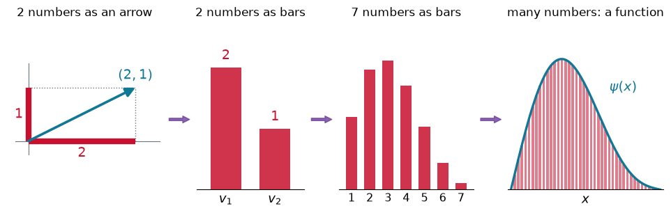

Fig. One vector, two pictures. The arrow $(2, 1)$ and its two components (red), then the same two numbers as bars. No arrow can show seven components, but seven bars can, and with many bars the tops trace a function.

So a function is a vector too, with one component per point. Pick $N$ grid points $x_1, x_2, \dots, x_N$ spaced $\Delta x$ apart and record the value of the function at each one, $\psi_j = \psi(x_j)$ . The function becomes a column of $N$ numbers.

# synced: function_vector
import numpy as np
import matplotlib.pyplot as plt
from matplotlib.animation import FuncAnimation
from IPython.display import HTML

TEAL, CARDINAL, GRAY, PURPLE, ORANGE = "#107895", "#C8102E", "#6c757d", "#6a3d9a", "#e07b00"
plt.rcParams.update({"axes.spines.top": False, "axes.spines.right": False})
xs = np.linspace(0, 1, 400)
f = lambda x: np.sin(np.pi * x) + 0.45 * np.sin(2 * np.pi * x)
N, dx = 7, 1 / 8
xj = dx * np.arange(1, N + 1); fj = f(xj)
fig = plt.figure(figsize=(9, 3.7))
gs = fig.add_gridspec(1, 3, width_ratios=[2.6, 0.5, 0.9], wspace=0.05)
ax, axa, axv = (fig.add_subplot(gs[0, j]) for j in range(3))
ax.plot(xs, f(xs), color=TEAL, lw=2.6, label=r"$\psi(x)$")
ax.vlines(xj, 0, fj, color=GRAY, lw=1, ls=":")
ax.plot(xj, fj, "o", color=CARDINAL, ms=8, zorder=5)
for j, (xv, fv) in enumerate(zip(xj, fj), start=1):
    ax.text(xv, fv + 0.09, rf"$\psi_{j}$", ha="center", fontsize=12, color=CARDINAL)
ax.plot([0, 0], [0, 1.55], color="k", lw=2.6); ax.plot([1, 1], [0, 1.55], color="k", lw=2.6)
ax.axhline(0, color=GRAY, lw=0.8)
ax.annotate("", xy=(xj[3], -0.14), xytext=(xj[2], -0.14), arrowprops=dict(arrowstyle="<->", color="k", lw=1.2))
ax.text((xj[2] + xj[3]) / 2, -0.2, r"$\Delta x$", ha="center", va="top", fontsize=13)
ax.set_xlim(-0.03, 1.03); ax.set_ylim(-0.42, 1.6)
ax.set_xticks(list(xj)); ax.set_xticklabels([rf"$x_{j}$" for j in range(1, N + 1)], fontsize=12)
ax.set_yticks([]); ax.spines["left"].set_visible(False); ax.spines["bottom"].set_visible(False)
ax.tick_params(length=0)
ax.set_title(r"a function, sampled at $N$ points spaced $\Delta x$ apart", loc="left", fontsize=12.5)
axa.axis("off")
axa.annotate("", xy=(0.95, 0.5), xytext=(0.05, 0.5), xycoords="axes fraction",
             arrowprops=dict(arrowstyle="simple,head_length=0.8,head_width=0.8,tail_width=0.3", color=PURPLE, alpha=0.8))
axv.axis("off"); axv.set_xlim(0, 1); axv.set_ylim(0, N + 1)
for j, fv in enumerate(fj, start=1):
    y = N + 0.5 - j
    axv.text(0.5, y, f"{fv:.2f}", ha="center", va="center", fontsize=13,
             bbox=dict(boxstyle="round,pad=0.25", fc="#fbeaec", ec=CARDINAL, lw=1))
    axv.text(0.02, y, rf"$\psi_{j}$", ha="left", va="center", fontsize=11, color=CARDINAL)
axv.plot([0.27, 0.22, 0.22, 0.27], [N + 0.35, N + 0.35, 0.15, 0.15], color="k", lw=1.4)
axv.plot([0.73, 0.78, 0.78, 0.73], [N + 0.35, N + 0.35, 0.15, 0.15], color="k", lw=1.4)
axv.set_title("a vector", fontsize=12.5)
fig.subplots_adjust(left=0.02, right=0.99, top=0.88, bottom=0.12)
plt.show()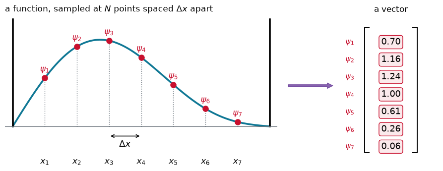

Fig. A wavefunction in a box sampled at seven interior points. The walls, where $\psi = 0$ , carry no unknowns. The seven samples, stacked in a column, are the vector that stands in for the function.

The letter $\psi$ now names three different things: the function, one sample of it, and the whole column of samples. Here they are with the grid symbols, in one place:

symbol	what it is
$\psi(x)$	the function: a value at every $x$
$N$	the number of grid points
$x_j$	grid point number $j$ , for $j = 1, \dots, N$
$\Delta x$	the spacing between neighboring grid points
$\psi_j = \psi(x_j)$	one number: the value of the function at $x_j$
$\lvert\psi\rangle$	all $N$ samples stacked in a column: the vector (Dirac notation, below)
$\langle\psi\rvert$	the same numbers written as a row, each one conjugated

Integrals become sums. As in a Riemann sum, each sample stands for a strip of width $\Delta x$ , so the $dx$ of the integral becomes $\Delta x$ . The inner product of two functions becomes the dot product of their vectors, times $\Delta x$ :

\int \phi^*\,\psi\,dx \;\approx\; \sum_{j} \phi_j^*\,\psi_j\,\Delta x, \qquad \int \lvert\psi\rvert^2\,dx = 1 \;\longrightarrow\; \sum_j \lvert\psi_j\rvert^2\,\Delta x = 1

(8)

The $\Delta x$ cannot be dropped: without it the sum grows with the number of points. For the box ground state $\sqrt{2/L}\,\sin(\pi x/L)$ sampled at $N$ interior points, $\sum_j \lvert\psi_j\rvert^2 = (N + 1)/L$ . Times $\Delta x = L/(N + 1)$ it is exactly 1, on any grid.

Step 2: multiplying by $x$ is a diagonal matrix¶

$\hat{x}$ multiplies the value at each point by that point’s own position, $(\hat{x}\psi)_j = x_j\,\psi_j$ . As a matrix acting on the vector, every entry off the diagonal is zero:

\hat{x}\,\psi \;\longrightarrow\; \begin{pmatrix} x_1 & 0 & 0 & 0 \\ 0 & x_2 & 0 & 0 \\ 0 & 0 & x_3 & 0 \\ 0 & 0 & 0 & x_4 \end{pmatrix} \begin{pmatrix} \psi_1 \\ \psi_2 \\ \psi_3 \\ \psi_4 \end{pmatrix} = \begin{pmatrix} x_1\psi_1 \\ x_2\psi_2 \\ x_3\psi_3 \\ x_4\psi_4 \end{pmatrix}

(9)

Any potential works the same way: $\hat{V}$ is the diagonal matrix of $V(x_1), \dots, V(x_N)$ . Multiplying by a function never mixes different points.

Step 3: derivatives compare neighbors¶

A derivative is a slope, and a slope needs two points. The centered difference uses the two neighbors of $x_j$ . For the second derivative, take the change between the slopes on either side, $s_+ = (\psi_{j+1} - \psi_j)/\Delta x$ and $s_- = (\psi_j - \psi_{j-1})/\Delta x$ , per unit length:

\psi'(x_j) \approx \frac{\psi_{j+1} - \psi_{j-1}}{2\Delta x}, \qquad \psi''(x_j) \approx \frac{s_+ - s_-}{\Delta x} = \frac{\psi_{j+1} - 2\psi_j + \psi_{j-1}}{\Delta x^2}

(10)

# synced: difference_stencils
import numpy as np
import matplotlib.pyplot as plt
from matplotlib.animation import FuncAnimation
from IPython.display import HTML

TEAL, CARDINAL, GRAY, PURPLE, ORANGE = "#107895", "#C8102E", "#6c757d", "#6a3d9a", "#e07b00"
plt.rcParams.update({"axes.spines.top": False, "axes.spines.right": False})
f = lambda x: 0.75 + 0.42 * np.sin(1.7 * x - 0.6) + 0.06 * x
df = lambda x: 0.42 * 1.7 * np.cos(1.7 * x - 0.6) + 0.06
xs = np.linspace(-0.2, 2.6, 300)
x0, dx = 1.15, 0.55
pts = np.array([x0 - dx, x0, x0 + dx]); fp = f(pts)
fig, (a1, a2) = plt.subplots(1, 2, figsize=(9.4, 4.0), gridspec_kw={"wspace": 0.1})
for ax in (a1, a2):
    ax.plot(xs, f(xs), color=GRAY, lw=2.2, alpha=0.8)
    ax.plot(pts, fp, "o", color=CARDINAL, ms=9, zorder=5)
    ax.set_xticks(pts); ax.set_xticklabels([r"$x_{j-1}$", r"$x_j$", r"$x_{j+1}$"], fontsize=12.5)
    ax.set_yticks([]); ax.spines["left"].set_visible(False)
    ax.set_xlim(-0.2, 2.6); ax.set_ylim(-0.62, 1.42)
t = np.array([x0 - 0.62, x0 + 0.62])
a1.plot(t, fp[1] + df(x0) * (t - x0), color="k", lw=1.6, ls="--", label=r"tangent at $x_j$: slope $\psi'(x_j)$")
sl = (fp[2] - fp[0]) / (2 * dx)
a1.plot(t, fp[1] + sl * (t - x0), color=PURPLE, lw=2.4, label=r"slope of the chord: $(\psi_{j+1} - \psi_{j-1})/2\Delta x$")
a1.plot([pts[0], pts[2]], [fp[0], fp[2]], color=PURPLE, lw=1.4, ls=":")
a1.legend(loc="lower center", frameon=False, fontsize=11.5)
a1.set_title("first derivative: the slope of the chord", loc="left", fontsize=12.5)
a2.plot(pts[:2], fp[:2], color=ORANGE, lw=2.6, label=r"$s_- = (\psi_j - \psi_{j-1})/\Delta x$")
a2.plot(pts[1:], fp[1:], color=TEAL, lw=2.6, label=r"$s_+ = (\psi_{j+1} - \psi_j)/\Delta x$")
a2.legend(loc="lower left", frameon=False, fontsize=11.5, bbox_to_anchor=(0.0, 0.13))
a2.text(0.01, 0.02, r"$\psi''(x_j) \approx \dfrac{s_+ - s_-}{\Delta x} = \dfrac{\psi_{j+1} - 2\psi_j + \psi_{j-1}}{\Delta x^2}$",
        transform=a2.transAxes, ha="left", va="bottom", fontsize=12.5)
a2.set_title("second derivative: how much the slope changes", loc="left", fontsize=12.5)
fig.subplots_adjust(left=0.01, right=0.99, top=0.91, bottom=0.09)
plt.show()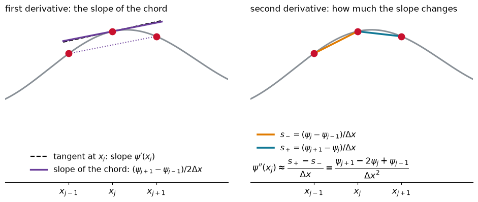

Fig. Derivatives from neighboring samples. Left: the chord through the two neighbors of $x_j$ is almost parallel to the tangent at $x_j$ , so its slope estimates $\psi'(x_j)$ . Right: the slope drops from $s_-$ to $s_+$ across $x_j$ ; the drop per unit length estimates $\psi''(x_j)$ , the curvature.

Each formula multiplies the samples at three neighboring points by fixed numbers: $-1, 0, 1$ (over $2\Delta x$ ) for the slope and $1, -2, 1$ (over $\Delta x^2$ ) for the curvature. Written as a row times a column, the curvature at point 2 is

\psi''(x_2) \approx \frac{1\cdot\psi_1 - 2\,\psi_2 + 1\cdot\psi_3}{\Delta x^2} = \frac{1}{\Delta x^2}\begin{pmatrix} 1 & -2 & 1 & 0 \end{pmatrix}\begin{pmatrix} \psi_1 \\ \psi_2 \\ \psi_3 \\ \psi_4 \end{pmatrix}

(11)

So the numbers of the formula are a row of a matrix. At point 3 the same numbers move one place to the right, $(0, 1, -2, 1)$ . Stacking one row per point, with $\psi = 0$ beyond the ends:

\frac{d}{dx} \;\longrightarrow\; D_1 = \frac{1}{2\Delta x}\begin{pmatrix} 0 & 1 & 0 & 0 \\ -1 & 0 & 1 & 0 \\ 0 & -1 & 0 & 1 \\ 0 & 0 & -1 & 0 \end{pmatrix}, \qquad \frac{d^2}{dx^2} \;\longrightarrow\; D_2 = \frac{1}{\Delta x^2}\begin{pmatrix} -2 & 1 & 0 & 0 \\ 1 & -2 & 1 & 0 \\ 0 & 1 & -2 & 1 \\ 0 & 0 & 1 & -2 \end{pmatrix}

(12)

Multiply the first row of $D_2$ into the vector: $(-2\psi_1 + \psi_2)/\Delta x^2$ . That is the curvature formula with $\psi_0 = 0$ , the value at the wall, so the boundary condition is built into the matrix.
Momentum is $\hat{p} = -i\hbar\,D_1$ : entries $-i\hbar/2\Delta x$ above the diagonal and $+i\hbar/2\Delta x$ below.

Example: the grid derivative of a plane wave

Apply the centered difference to the samples of a plane wave, $\psi_j = e^{ikx_j}$ :

\frac{\psi_{j+1} - \psi_{j-1}}{2\Delta x} = \frac{e^{ik(x_j + \Delta x)} - e^{ik(x_j - \Delta x)}}{2\Delta x} = \frac{e^{ik\Delta x} - e^{-ik\Delta x}}{2\Delta x}\,e^{ikx_j} = \frac{i\sin(k\Delta x)}{\Delta x}\,\psi_j

(13)

The sampled plane wave is an eigenvector of the derivative matrix, just as $e^{ikx}$ is an eigenfunction of $d/dx$ (away from the ends of the grid). The eigenvalue $i\sin(k\Delta x)/\Delta x$ approaches the exact $ik$ when the grid is fine, $k\Delta x \ll 1$ . Multiplied by $-i\hbar$ , the momentum matrix returns $\hbar\sin(k\Delta x)/\Delta x \approx \hbar k$ , the de Broglie momentum. The grid works when it has many points per wavelength.

Step 4: the Hamiltonian is a matrix¶

Put the pieces together: $\hat{H} = -\frac{\hbar^2}{2m}\frac{d^2}{dx^2} + V(x)$ becomes $H = -\frac{\hbar^2}{2m}D_2 + V$ . The constants in front of $D_2$ collect into one symbol, $\varepsilon = \hbar^2/2m\Delta x^2$ , which is only a unit of energy:

H = \begin{pmatrix} 2\varepsilon + V_1 & -\varepsilon & 0 & 0 \\ -\varepsilon & 2\varepsilon + V_2 & -\varepsilon & 0 \\ 0 & -\varepsilon & 2\varepsilon + V_3 & -\varepsilon \\ 0 & 0 & -\varepsilon & 2\varepsilon + V_4 \end{pmatrix}, \qquad \varepsilon = \frac{\hbar^2}{2m\,\Delta x^2}

(14)

Read it as a picture: the potential energy sits on the diagonal, one value per point, and the kinetic energy couples each point to its neighbors through $-\varepsilon$ . This is the same structure as the Hückel matrix that chemists use for $\pi$ electrons hopping between carbon atoms (Problem 6).

Example: a particle in a box with three grid points

Divide a box of length $L$ into four intervals, $\Delta x = L/4$ . The wavefunction vanishes at the two walls, which leaves three interior points, $x = L/4$ , $L/2$ and $3L/4$ . With $V = 0$ inside,

H = \varepsilon\begin{pmatrix} 2 & -1 & 0 \\ -1 & 2 & -1 \\ 0 & -1 & 2 \end{pmatrix}, \qquad \varepsilon = \frac{\hbar^2}{2m\,\Delta x^2} = \frac{8\hbar^2}{mL^2}

(16)

Write $E = \lambda\varepsilon$ and solve $\det(H/\varepsilon - \lambda I) = 0$ . Go along the first row: each entry times the $2\times 2$ determinant that is left when its row and column are crossed out, with the signs $+\,-\,+$ :

(2-\lambda)\underbrace{\big[(2-\lambda)^2 - 1\big]}_{\text{row 1, column 1 crossed out}} - (-1)\underbrace{\big[-(2-\lambda)\big]}_{\text{row 1, column 2 crossed out}} + 0 = (2-\lambda)\big[(2-\lambda)^2 - 2\big] = 0

(17)

The product vanishes when $\lambda = 2$ or $(2 - \lambda)^2 = 2$ , so $\lambda = 2 - \sqrt{2},\ 2,\ 2 + \sqrt{2}$ . They add up to the trace, 6, and multiply to the determinant, 4. The lowest level is $E_1 = (2 - \sqrt{2})\,\varepsilon = 4.69\,\hbar^2/mL^2$ , within 5 percent of the exact $\pi^2\hbar^2/2mL^2 = 4.93\,\hbar^2/mL^2$ .

A row-times-column check confirms the ground state. Sample the exact ground state $\sin(\pi x/L)$ at the three points, $\big(\sin\tfrac{\pi}{4}, \sin\tfrac{\pi}{2}, \sin\tfrac{3\pi}{4}\big) \propto (1, \sqrt{2}, 1)$ :

\begin{pmatrix} 2 & -1 & 0 \\ -1 & 2 & -1 \\ 0 & -1 & 2 \end{pmatrix}\begin{pmatrix} 1 \\ \sqrt{2} \\ 1 \end{pmatrix} = \begin{pmatrix} 2 - \sqrt{2} \\ 2\sqrt{2} - 2 \\ 2 - \sqrt{2} \end{pmatrix} = (2 - \sqrt{2})\begin{pmatrix} 1 \\ \sqrt{2} \\ 1 \end{pmatrix}

(18)

The middle entry works because $2\sqrt{2} - 2 = (2 - \sqrt{2})\sqrt{2}$ . The grid’s ground state is the exact sine, sampled at the grid points.

# synced: box_grid_states
import numpy as np
import matplotlib.pyplot as plt
from matplotlib.animation import FuncAnimation
from IPython.display import HTML

TEAL, CARDINAL, GRAY, PURPLE, ORANGE = "#107895", "#C8102E", "#6c757d", "#6a3d9a", "#e07b00"
plt.rcParams.update({"axes.spines.top": False, "axes.spines.right": False})
xs = np.linspace(0, 1, 300)                                 # hbar = m = L = 1
fig = plt.figure(figsize=(9.4, 4.0))
gs = fig.add_gridspec(3, 3, width_ratios=[1.15, 0.42, 1], hspace=0.25, wspace=0.12)
N, dx = 3, 0.25
xg = np.array([0, 0.25, 0.5, 0.75, 1.0])
H = (2 * np.eye(N) - np.eye(N, k=1) - np.eye(N, k=-1)) / (2 * dx**2)
Eg, V = np.linalg.eigh(H)
for r in range(3):
    ax = fig.add_subplot(gs[r, 0])
    n = r + 1
    v = V[:, r] / np.sqrt(dx); v = v * np.sign(v[0])         # normalized as a function, first point positive
    ax.plot(xs, np.sqrt(2) * np.sin(n * np.pi * xs), color=GRAY, lw=1.8, alpha=0.7)
    ax.plot(xg, np.concatenate([[0], v, [0]]), "-o", color=CARDINAL, lw=1.6, ms=7)
    ax.axhline(0, color=GRAY, lw=0.6)
    ax.plot([0, 0], [-1.6, 1.6], color="k", lw=2); ax.plot([1, 1], [-1.6, 1.6], color="k", lw=2)
    ax.set_xlim(-0.03, 1.03); ax.set_ylim(-1.75, 1.75); ax.axis("off")
    axt = fig.add_subplot(gs[r, 1]); axt.axis("off")
    axt.text(0.05, 0.5, rf"$n = {n}$: $E = {Eg[r]:.2f}$" + "\n" + rf"exact: ${(n * np.pi)**2 / 2:.2f}$", fontsize=11.5,
             va="center", transform=axt.transAxes)
    if r == 0:
        ax.set_title("3 grid points: eigenvectors (dots) vs exact states", loc="left", fontsize=12.5)
axl = fig.add_subplot(gs[:, 2])
cols = [(3, CARDINAL), (10, PURPLE), (30, TEAL)]
for k, (Ng, col) in enumerate(cols):
    dxg = 1 / (Ng + 1)
    En = (1 - np.cos(np.arange(1, min(Ng, 4) + 1) * np.pi * dxg)) / dxg**2
    axl.hlines(En, k - 0.32, k + 0.32, color=col, lw=3)
Ex = (np.arange(1, 5) * np.pi)**2 / 2
axl.hlines(Ex, 3 - 0.32, 3 + 0.32, color="k", lw=3)
for e in Ex:
    axl.axhline(e, color=GRAY, lw=0.6, ls=":", zorder=0)
axl.set_xticks([0, 1, 2, 3]); axl.set_xticklabels([r"$N = 3$", r"$N = 10$", r"$N = 30$", "exact"], fontsize=12)
axl.yaxis.tick_right(); axl.yaxis.set_label_position("right")
axl.spines["left"].set_visible(False); axl.spines["right"].set_visible(True)
axl.set_ylabel(r"energy  ($\hbar^2/mL^2$)", fontsize=12); axl.tick_params(axis="y", labelsize=11)
axl.set_xlim(-0.6, 3.6); axl.set_ylim(0, 85)
axl.set_title("more points: closer to exact", loc="left", fontsize=12.5)
fig.subplots_adjust(left=0.01, right=0.99, top=0.9, bottom=0.09)
fig.subplots_adjust(right=0.93)
plt.show()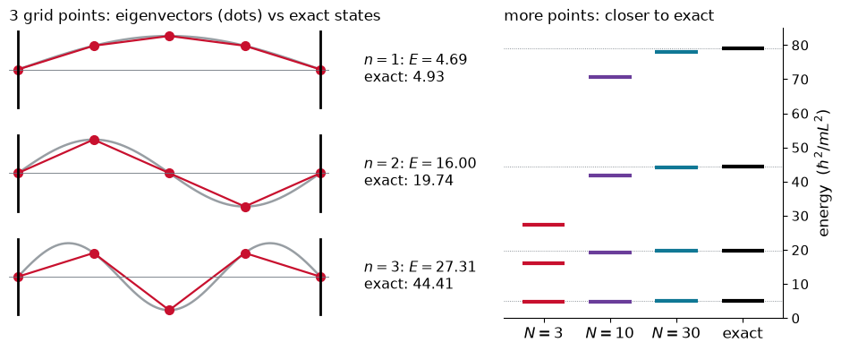

Fig. Left: the three eigenvectors of the three-point box (dots, joined by straight lines) on top of the exact box states (gray). Each is the exact sine sampled at the grid points. Right: the levels of grids with 3, 10 and 30 points against the exact ones, in units of $\hbar^2/mL^2$ . More points give more levels, and each converges to the exact value from below. The top levels of a coarse grid are the least accurate, because their short wavelengths have few points per wavelength.

Example: five lines of numpy to solve the 1D Schrödinger equation

With 400 points instead of 3, the eigenvalue problem is too big for a determinant by hand, and numpy solves it in one call. Here is the particle on a spring whose levels you hunted with the trial-energy slider in The Schrödinger Equation, in units with $\hbar = m = \omega = 1$ :

import numpy as np

N = 400                                       # grid points
x = np.linspace(-8, 8, N); dx = x[1] - x[0]
D2 = (np.eye(N, k=1) - 2 * np.eye(N) + np.eye(N, k=-1)) / dx**2   # second derivative
H = -0.5 * D2 + np.diag(0.5 * x**2)           # kinetic + potential energy

E, psi = np.linalg.eigh(H)                    # eigenvalues and eigenvectors of a Hermitian matrix
print(np.round(E[:5], 4))                     # exact: 0.5 1.5 2.5 3.5 4.5

[0.4999 1.4997 2.4993 3.4987 4.4979]

The levels come out $0.5, 1.5, 2.5, \dots$ in units of $\hbar\omega$ , to three or four digits. This evenly spaced ladder is the vibrating bond of Chapter 4. The columns of psi are the wavefunctions.
eigh is numpy’s eigensolver for Hermitian matrices. Why the physics hands us only Hermitian matrices is the subject of Operators 2.

Dirac notation¶

Integrals and matrices are two ways of writing the same objects. Dirac’s notation writes them once, and it reads like matrix algebra: a ket is a column, a bra is a row, and a row times a column is a number.

Kets and bras¶

A state is a ket $\lvert\psi\rangle$ : on the grid, the column of samples from Step 1. Its partner, the bra $\langle\psi\rvert$ , is the same numbers written as a row, each one conjugated:

\lvert\psi\rangle = \begin{pmatrix} \psi_1 \\ \psi_2 \\ \vdots \end{pmatrix}, \qquad \langle\psi\rvert = \begin{pmatrix} \psi_1^* & \psi_2^* & \cdots \end{pmatrix}

(19)

A bra next to a ket is row times column: multiply matching entries and add. The result is a single number, the inner product. For sampled functions the sum also carries the $\Delta x$ of Step 1, because it stands for an integral; ordinary vectors, like the two-component examples below, have no $\Delta x$ :

\langle \phi \vert \psi \rangle = \sum_j \phi_j^*\,\psi_j\,\Delta x \;\longrightarrow\; \int \phi^*\,\psi\,dx

(20)

Example: why the bra is conjugated

Take the two-component ket $\lvert\psi\rangle = \begin{pmatrix} 1 \\ i \end{pmatrix}$ . Its bra is $\langle\psi\rvert = (1,\ -i)$ , so

\langle \psi \vert \psi \rangle = 1\cdot 1 + (-i)(i) = 1 + 1 = 2

(21)

a real, positive length squared. Without the conjugate the same product would be $1\cdot 1 + i\cdot i = 0$ : a nonzero vector of zero length. Conjugating the bra makes every $\langle \psi \vert \psi \rangle$ real and positive, which is what allows $\lvert\psi\rvert^2$ to be a probability density.

One consequence is used all the time: a constant $c$ comes out of a ket unchanged but out of a bra conjugated. The star in the integral does it:

\begin{aligned} \langle \phi \vert c\,\psi \rangle &= \int \phi^*\,(c\,\psi)\,dx = c\,\langle \phi \vert \psi \rangle \\ \langle c\,\phi \vert \psi \rangle &= \int (c\,\phi)^*\,\psi\,dx = c^*\langle \phi \vert \psi \rangle \end{aligned}

(22)

Sandwiches: matrix elements¶

An operator acts on a ket, $\hat{A}\lvert\psi\rangle$ , and gives a new ket: on the grid, the matrix times the column. Put a bra in front and the result is a number, the matrix element: row times matrix times column.

\langle\phi\vert\hat{A}\vert\psi\rangle = \int\phi^*\,\hat{A}\psi\,dx

(23)

Count the shapes to see what any product gives. A bra is a row, an operator a square, a ket a column. In a product the inner sizes must match, and the outer sizes give the size of the result.

# synced: dirac_shapes
import numpy as np
import matplotlib.pyplot as plt
from matplotlib.animation import FuncAnimation
from IPython.display import HTML

TEAL, CARDINAL, GRAY, PURPLE, ORANGE = "#107895", "#C8102E", "#6c757d", "#6a3d9a", "#e07b00"
from matplotlib.patches import Rectangle
plt.rcParams.update({"axes.spines.top": False, "axes.spines.right": False})
W, Ht = 9.6, 2.6                                            # draw in inches: one data unit = one inch
fig = plt.figure(figsize=(W, Ht))
ax = fig.add_axes([0, 0, 1, 1]); ax.set_xlim(0, W); ax.set_ylim(0, Ht); ax.axis("off")
s, n, ym = 0.19, 4, 1.33                                    # cell size, N, middle line of the shapes
look = {"bra": ("#fdf0e0", ORANGE), "op": ("#f1ecf7", PURPLE), "ket": ("#e3f1f5", TEAL), "num": ("#fbeaec", CARDINAL)}

def shape(x0, rows, cols, kind, below, size):               # rows x cols cells, left edge x0, centred on the line ym
    fc, ec = look[kind]
    for r in range(rows):
        for c in range(cols):
            ax.add_patch(Rectangle((x0 + c * s, ym + (rows / 2 - 1 - r) * s), s, s, fc=fc, ec=ec, lw=1.2))
    ax.text(x0 + cols * s / 2, ym - n * s / 2 - 0.34, below, ha="center", va="baseline", fontsize=14, color=ec)
    ax.text(x0 + cols * s / 2, ym + n * s / 2 + 0.1, size, ha="center", va="bottom", fontsize=11.5, color=GRAY)

eq = lambda x: ax.text(x, ym, "=", ha="center", va="center", fontsize=18)
panels = [(1.35, "inner product", "a number"), (4.15, "an operator acts", "a new ket"), (7.45, "a matrix element", "a number")]
for xc, title, note in panels:
    ax.text(xc, 2.33, title, ha="center", va="center", fontsize=13)
    ax.text(xc, 0.27, note, ha="center", va="center", fontsize=12.5, color=GRAY)
for xv in (2.75, 5.55):
    ax.plot([xv, xv], [0.15, 2.45], color="#dee2e6", lw=1)
shape(0.4, 1, n, "bra", r"$\langle\phi|$", r"$1\times 4$")                       # row times column: a number
shape(1.33, n, 1, "ket", r"$|\psi\rangle$", r"$4\times 1$")
eq(1.8); shape(2.0, 1, 1, "num", r"$\langle\phi|\psi\rangle$", r"$1\times 1$")
shape(3.2, n, n, "op", r"$\hat{A}$", r"$4\times 4$")                              # matrix times column: a column
shape(4.13, n, 1, "ket", r"$|\psi\rangle$", r"$4\times 1$")
eq(4.6); shape(4.8, n, 1, "ket", r"$\hat{A}|\psi\rangle$", r"$4\times 1$")
shape(6.0, 1, n, "bra", r"$\langle\phi|$", r"$1\times 4$")                       # row, matrix, column: a number
shape(6.93, n, n, "op", r"$\hat{A}$", r"$4\times 4$")
shape(7.86, n, 1, "ket", r"$|\psi\rangle$", r"$4\times 1$")
eq(8.33); shape(8.53, 1, 1, "num", r"$\langle\phi|\hat{A}|\psi\rangle$", r"$1\times 1$")
plt.show()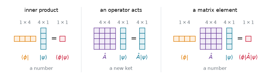

Fig. Count the shapes. A bra is a $1\times N$ row, an operator an $N\times N$ square, a ket an $N\times 1$ column (here $N = 4$ ). Row times column is a single number; a matrix times a column is a new column, a ket; row times matrix times column is again a single number, the matrix element.

The name is literal: the matrix is the filling between a bra and a ket. Put the unit vectors $\mathbf{e}_1 = (1, 0)$ and $\mathbf{e}_2 = (0, 1)$ on the outside and the sandwich picks out a single entry.
Take $A = \begin{pmatrix} 2 & 1 \\ 1 & 2 \end{pmatrix}$ and do it in two steps, the ket first and then the bra:

\begin{aligned} A\mathbf{e}_2 &= \begin{pmatrix} 2 & 1 \\ 1 & 2 \end{pmatrix}\begin{pmatrix} 0 \\ 1 \end{pmatrix} = \begin{pmatrix} 1 \\ 2 \end{pmatrix} \\ \langle \mathbf{e}_1 \vert A \vert \mathbf{e}_2 \rangle &= \begin{pmatrix} 1 & 0 \end{pmatrix}\begin{pmatrix} 1 \\ 2 \end{pmatrix} = 1 = A_{12} \end{aligned}

(24)

The ket picked out column 2 of the matrix, and the bra then picked out the first entry of that column. In general, the sandwich of the unit vectors $\mathbf{e}_j$ and $\mathbf{e}_k$ is the entry in row $j$ and column $k$ :

A_{jk} = \langle \mathbf{e}_j \vert A \vert \mathbf{e}_k \rangle

(25)

In a basis of functions instead of grid points, the same sandwich builds the matrices that quantum chemistry programs diagonalize: $H_{mn} = \langle \phi_m \vert \hat{H} \vert \phi_n \rangle$ for a set of orbitals $\phi_n$ (Hückel Theory).

Diagonalizing a Hamiltonian¶

The entries of a matrix depend on the axes you write it in; the operator does not. Turn the axes to perpendicular unit vectors $\mathbf{u}_1, \mathbf{u}_2, \dots$ and each entry becomes a sandwich, $A'_{mn} = \langle \mathbf{u}_m \vert A \vert \mathbf{u}_n \rangle$ . A Matrix in New Axes in Appendix A lets you turn the axes yourself and watch the entries change.

This is what diagonalizing a Hamiltonian means: finding the axes, its eigenvectors, in which $H$ is diagonal. The diagonal then lists the energies. For the three-point box it holds $2 - \sqrt{2}$ , 2 and $2 + \sqrt{2}$ in units of $\varepsilon$ , the energies found by hand above.
numpy finds the axes in one call. E, U = np.linalg.eigh(H) returns the eigenvectors as the columns of U, and U.T @ H @ U is $H$ in those axes: diagonal, with E on the diagonal. A complex matrix needs the conjugate in the bra, U.conj().T @ H @ U. Measurement uses the same idea to expand a wavefunction along the eigenfunctions of an operator.

One language, three dialects¶

	integral	Dirac	numpy on a grid
inner product	$\int \phi^*\psi\,dx$	$\langle \phi \vert \psi \rangle$	`np.vdot(phi, psi) * dx`
normalization	$\int \lvert\psi\rvert^2 dx = 1$	$\langle \psi \vert \psi \rangle = 1$	`np.vdot(psi, psi) * dx`
operator acts	$\hat{A}\psi(x)$	$\hat{A}\lvert\psi\rangle$	`A @ psi`
matrix element	$\int \phi^*\hat{A}\psi\,dx$	$\langle \phi \vert \hat{A} \vert \psi \rangle$	`np.vdot(phi, A @ psi) * dx`
eigenvalue problem	$\hat{A}\phi_n = a_n\phi_n$	$\hat{A}\lvert n\rangle = a_n\lvert n\rangle$	`a, phi = np.linalg.eigh(A)`
matrix in new axes	$A'_{mn} = \int \phi_m^*\hat{A}\phi_n\,dx$	$A'_{mn} = \langle \phi_m \vert \hat{A} \vert \phi_n \rangle$	`U.conj().T @ A @ U * dx` (columns of `U`: the $\phi_n$ )

np.vdot conjugates its first argument, which is exactly what the bra does. The factor dx is the grid spacing $\Delta x$ : it turns the sum over grid points into the integral.
The table grows in the next three lectures: adjoints and commutators in Operators 2, expansion coefficients in Measurement, time evolution in Time Dependence.

Two matrix properties to watch¶

Here are $\hat{x}$ , $\hat{p}$ and $\hat{H}$ for a particle on a spring on an 8-point grid, as color maps. At any size they keep the same pattern:

# synced: grid_operators
import numpy as np
import matplotlib.pyplot as plt
from matplotlib.animation import FuncAnimation
from IPython.display import HTML

TEAL, CARDINAL, GRAY, PURPLE, ORANGE = "#107895", "#C8102E", "#6c757d", "#6a3d9a", "#e07b00"
from matplotlib.colors import LinearSegmentedColormap
plt.rcParams.update({"axes.spines.top": False, "axes.spines.right": False})
div = LinearSegmentedColormap.from_list("div", [TEAL, "white", CARDINAL])
N = 8                                                       # hbar = m = 1, V = x^2/2 on 8 points
x = np.linspace(-2, 2, N); dx = x[1] - x[0]
up, dn = np.eye(N, k=1), np.eye(N, k=-1)
X = np.diag(x)
P = -1j * (up - dn) / (2 * dx)                              # p = -i d/dx as a centered difference
H = -0.5 * (up - 2 * np.eye(N) + dn) / dx**2 + np.diag(0.5 * x**2)
panels = [(X, r"$\hat{x}$", "grid positions on the diagonal\nreal, symmetric"),
          (P.imag, r"$\hat{p}$  (imaginary part)", r"$\mp i\hbar/2\Delta x$ next to the diagonal" + "\nimaginary, antisymmetric"),
          (H, r"$\hat{H}$", "$V$ on the diagonal, neighbors linked\nreal, symmetric")]
fig, axs = plt.subplots(1, 3, figsize=(9.6, 3.8))
for ax, (M, title, note) in zip(axs, panels):
    m = np.abs(M).max()
    ax.imshow(M, cmap=div, vmin=-m, vmax=m)
    ax.set_xticks(np.arange(-0.5, N, 1), minor=True); ax.set_yticks(np.arange(-0.5, N, 1), minor=True)
    ax.grid(which="minor", color="white", lw=1.5)
    ax.tick_params(which="both", length=0, labelbottom=False, labelleft=False)
    for sp in ax.spines.values():
        sp.set_visible(False)
    ax.set_title(title, fontsize=14)
    ax.set_xlabel(note, fontsize=11.5, linespacing=1.4)
fig.suptitle(r"each matrix equals its conjugate transpose: $A^\dagger = A$", fontsize=13, y=0.98)
fig.subplots_adjust(left=0.02, right=0.98, top=0.83, bottom=0.17, wspace=0.18)
plt.show()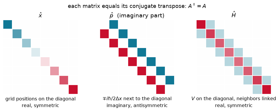

Fig. Position, momentum and energy of a particle on a spring, on a grid of 8 points. Color shows the sign and size of each entry (teal negative, red positive, white zero). Each matrix equals its own conjugate transpose, the defining property of a Hermitian matrix (Operators 2); momentum manages it with an imaginary, antisymmetric pattern.

Mirror symmetry. Each of these matrices equals its own mirror image across the diagonal, after conjugating the entries. Matrices like this are called Hermitian, and Operators 2 shows why every observable must be one: it guarantees real eigenvalues.
Order. Matrix products depend on the order, $AB \neq BA$ in general, and on the grid $XP \neq PX$ . The difference, the commutator, decides which observables can be sharp at the same time (Operators 2).

Problems¶

Problem 1: Linear or not?¶

Decide which of these operators are linear: (a) $\hat{A}f = f + x$ , (b) $\hat{B}f = x^2\,\dfrac{d^2f}{dx^2}$ , (c) $\hat{C}f = \displaystyle\int_0^x f(y)\,dy$ , (d) $\hat{D}f = e^{f}$ .

Solution

(a) Not linear. $\hat{A}(2f) = 2f + x$ , but $2\hat{A}f = 2f + 2x$ . Adding something that does not depend on $f$ always breaks linearity.
(b) Linear. The second derivative of a sum is the sum of the second derivatives, and multiplying by $x^2$ keeps constants and sums intact.
(c) Linear. The integral of $c_1f_1 + c_2f_2$ is $c_1\int f_1 + c_2\int f_2$ .
(d) Not linear. $e^{f_1 + f_2} = e^{f_1}e^{f_2}$ , a product rather than a sum.

Problem 2: Eigenvectors by hand¶

Find the eigenvalues and eigenvectors of $B = \begin{pmatrix} 2 & 2 \\ 2 & -1 \end{pmatrix}$ . Check them against the trace and the determinant, and check that the two eigenvectors are perpendicular.

Solution

\det(B - \lambda I) = (2 - \lambda)(-1 - \lambda) - 4 = \lambda^2 - \lambda - 6 = (\lambda - 3)(\lambda + 2) = 0 \quad\Longrightarrow\quad \lambda = 3,\ -2

(27)

For $\lambda = 3$ the first row of $(B - 3I)\mathbf{v} = 0$ reads $-v_1 + 2v_2 = 0$ , so $\mathbf{v} \propto (2, 1)$ . For $\lambda = -2$ it reads $4v_1 + 2v_2 = 0$ , so $\mathbf{v} \propto (1, -2)$ . Checks: $3 + (-2) = 1$ is the trace $2 + (-1)$ , and $3 \times (-2) = -6$ is the determinant $2\cdot(-1) - 2\cdot 2$ . The dot product $(2, 1)\cdot(1, -2) = 0$ , so the eigenvectors are perpendicular, a property of every symmetric matrix that Operators 2 explains.

Problem 3: Two orbitals, one matrix¶

In Hückel theory the two $p$ orbitals of ethylene are described by $H = \begin{pmatrix} \alpha & \beta \\ \beta & \alpha \end{pmatrix}$ , where $\alpha$ is the energy of an electron on one carbon and $\beta < 0$ couples the two. Find the energies and the normalized eigenvectors. Which combination is lower in energy?

Solution

$\det(H - EI) = (\alpha - E)^2 - \beta^2 = 0$ , so $\alpha - E = \pm\beta$ and $E = \alpha + \beta$ or $E = \alpha - \beta$ . For $E = \alpha + \beta$ the first row of $(H - EI)\mathbf{v} = 0$ reads $-\beta v_1 + \beta v_2 = 0$ , so $\mathbf{v} = (1, 1)/\sqrt{2}$ ; for $E = \alpha - \beta$ , $\mathbf{v} = (1, -1)/\sqrt{2}$ . Since $\beta < 0$ , $\alpha + \beta$ is the lower energy: the in-phase combination $(1, 1)/\sqrt{2}$ is the bonding orbital, and the out-of-phase $(1, -1)/\sqrt{2}$ , with a node between the carbons, is antibonding. The eigenvectors do not depend on $\alpha$ or $\beta$ at all; the symmetry of the molecule fixes them.

Problem 4: Position as a matrix in the box basis¶

Use the box states $\psi_n = \sqrt{2/L}\,\sin(n\pi x/L)$ as a basis and build the $3\times 3$ matrix $x_{mn} = \langle \psi_m \vert \hat{x} \vert \psi_n \rangle$ , $m, n = 1, 2, 3$ , with numpy on a grid. Is the matrix symmetric? Which entries vanish?

Solution

import numpy as np
L = 1.0
x = np.linspace(0, L, 2001); dx = x[1] - x[0]
psi = np.array([np.sqrt(2 / L) * np.sin(n * np.pi * x / L) for n in (1, 2, 3)])
X = np.array([[np.sum(psi[m] * x * psi[n]) * dx for n in range(3)] for m in range(3)])
print(np.round(X, 4))   # [[ 0.5 -0.1801 0. ] [-0.1801 0.5 -0.1945] [ 0. -0.1945 0.5]]

Each diagonal entry is $\langle x \rangle = L/2$ , because every box state is symmetric about the middle of the box. The matrix is symmetric, $x_{mn} = x_{nm}$ , as a real operator in a real basis must be. The entries $x_{13} = x_{31}$ vanish: write $x = (x - L/2) + L/2$ ; the $L/2$ part gives $\tfrac{L}{2}\langle \psi_1 \vert \psi_3 \rangle = 0$ , and in the other part $\psi_1\psi_3$ is symmetric about $L/2$ while $x - L/2$ is antisymmetric, so the two halves of the integral cancel.

Problem 5: A rotation has no real eigenvectors¶

The matrix $R = \begin{pmatrix} \cos\theta & -\sin\theta \\ \sin\theta & \cos\theta \end{pmatrix}$ turns every arrow by the angle $\theta$ . Apply it to $(1, 0)$ and $(0, 1)$ for $\theta = 90^\circ$ and sketch the results. Then show that its eigenvalues are $\lambda = \cos\theta \pm i\sin\theta = e^{\pm i\theta}$ , find the eigenvectors, and say for which angles the eigenvalues are real. Why does the picture make the answer obvious?

Problem 6: Butadiene as a matrix¶

In Hückel theory (Chapter 8) the $\pi$ electrons of butadiene are described by the matrix

H = \begin{pmatrix} \alpha & \beta & 0 & 0 \\ \beta & \alpha & \beta & 0 \\ 0 & \beta & \alpha & \beta \\ 0 & 0 & \beta & \alpha \end{pmatrix}

(28)

where $\alpha$ is the energy of an electron on one carbon and $\beta < 0$ couples neighbors. Set $\alpha = 0$ , $\beta = -1$ and use np.linalg.eigh to find the eigenvalues and eigenvectors. Check that the eigenvalues are real (you should find $\pm 1.618$ and $\pm 0.618$ ) and that the eigenvectors are orthonormal. Draw each eigenvector as four bars, one per carbon, and count the sign changes. Compare with the particle-in-a-box states of butadiene in Particle in a Box.

Problem 7: Brackets on a grid¶

Sample the box states $\psi_1$ and $\psi_2$ ( $L = 1$ ) on $N$ interior grid points and compute $\langle \psi_1 \vert \psi_1 \rangle$ , $\langle \psi_2 \vert \psi_2 \rangle$ and $\langle \psi_1 \vert \psi_2 \rangle$ with np.vdot(...) * dx. How close are they to 1, 1 and 0 for $N = 5$ , 20 and 100? Then multiply $\psi_2$ by $c = 2i$ and confirm that $\langle c\,\psi_2 \vert \psi_2 \rangle = c^*\langle \psi_2 \vert \psi_2 \rangle$ while $\langle \psi_2 \vert c\,\psi_2 \rangle = c\,\langle \psi_2 \vert \psi_2 \rangle$ .

Problem 8: How many points per wavelength?¶

Adapt the five lines of numpy to the particle in a box: $V = 0$ on $N$ interior points, $\hbar = m = L = 1$ , exact levels $E_n = n^2\pi^2/2$ . For $n = 1$ , 5 and 10, find how many points you need for a 1 percent error, and express each answer as points per wavelength, $2(N + 1)/n$ . What rule of thumb do you find?

The rules of the game¶

Operators act on functions¶

Linear operators¶

Matrices act on vectors¶

From operators to matrices¶

Step 1: a function becomes a vector¶

Step 2: multiplying by xxx is a diagonal matrix¶

Step 3: derivatives compare neighbors¶

Step 4: the Hamiltonian is a matrix¶

Dirac notation¶

Kets and bras¶

Sandwiches: matrix elements¶

Diagonalizing a Hamiltonian¶

One language, three dialects¶

Two matrix properties to watch¶

Problems¶

Problem 1: Linear or not?¶

Problem 2: Eigenvectors by hand¶

Problem 3: Two orbitals, one matrix¶

Problem 4: Position as a matrix in the box basis¶

Problem 5: A rotation has no real eigenvectors¶

Problem 6: Butadiene as a matrix¶

Problem 7: Brackets on a grid¶

Problem 8: How many points per wavelength?¶

Step 2: multiplying by $x$ is a diagonal matrix¶