Classical vs Quantum particle in a box
The particle in a box is a toy model of an electron (or atom, molecule, or small quantum object) trapped in some region of space .
The positional information of a quantum “particle” is described by a quantum wave function , which is obtained by solving the Schrödinger equation with boundary conditions.
Wave functions are standing waves, just as in the vibrating guitar string problem, with one major difference: a quantum wave function has a probabilistic meaning and hence is completely different from the classical notion of a “wave”.
According to classical mechanics, in the absence of any attractive interactions the particle bounces back and forth between the walls with constant speed. We therefore expect to find it with equal probability at all locations .
According to quantum mechanics, the quantum particle in the box is found in some regions with high probability and in others with little or zero probability.
Source
# synced: box_bounce
import numpy as np
import matplotlib.pyplot as plt
from matplotlib.animation import FuncAnimation
from IPython.display import HTML
TEAL, CARDINAL, GRAY, PURPLE, ORANGE = "#107895", "#C8102E", "#6c757d", "#6a3d9a", "#e07b00"
plt.rcParams.update({"axes.spines.top": False, "axes.spines.right": False})
rng = np.random.default_rng(5)
xc = rng.random(4000) # classical: snapshots at random times
cand = rng.random(16000)
xq = cand[rng.random(16000) < np.sin(3 * np.pi * cand) ** 2][:4000] # quantum: samples of |psi_3|^2
yj = rng.random(4000)
counts = np.unique(np.round(np.geomspace(1, 4000, 44)).astype(int))
counts = np.concatenate([counts, np.full(8, counts[-1])])
edges = np.linspace(0, 1, 31); mid = 0.5 * (edges[1:] + edges[:-1]); dx = edges[1] - edges[0]
xs = np.linspace(0, 1, 300)
fig, axes = plt.subplots(2, 2, figsize=(8, 3.9), sharex=True,
gridspec_kw={"height_ratios": [1, 2.2], "hspace": 0.12, "wspace": 0.1})
(ta, tb), (ha, hb) = axes
for ax in (ta, tb):
ax.axvline(0, color="k", lw=3); ax.axvline(1, color="k", lw=3)
ax.set_ylim(0, 1); ax.set_yticks([]); ax.spines["left"].set_visible(False); ax.tick_params(bottom=False)
ta.set_title("classical: a ball bouncing at constant speed", loc="left", fontsize=10.5)
tb.set_title(r"quantum, $n = 3$: each dot is one detection", loc="left", fontsize=10.5)
(trail,) = ta.plot([], [], "o", color=ORANGE, ms=9, alpha=0.25)
(ball,) = ta.plot([], [], "o", color=ORANGE, ms=12)
scat = tb.scatter([], [], s=5, color=TEAL, alpha=0.6, lw=0)
bars_c = ha.bar(mid, 0 * mid, width=0.92 * dx, color=ORANGE, alpha=0.5)
bars_q = hb.bar(mid, 0 * mid, width=0.92 * dx, color=TEAL, alpha=0.5)
(pc,) = ha.plot([], [], color=GRAY, lw=2.4, ls="--", label=r"flat: $1/L$")
(pq,) = hb.plot([], [], color=CARDINAL, lw=2.4, label=r"$|\psi_3(x)|^2$")
for ax in (ha, hb):
ax.set_xlim(-0.02, 1.02); ax.set_yticks([])
ax.set_xticks([0, 0.5, 1]); ax.set_xticklabels(["0", "L/2", "L"]); ax.set_xlabel("position x")
ax.legend(loc="upper right", frameon=False, fontsize=9.5)
ha.set_ylabel("times caught here")
fig.subplots_adjust(left=0.05, right=0.99, top=0.84, bottom=0.13)
sup = fig.suptitle("", fontsize=11.5)
tri = lambda s: 0.04 + 0.92 * (1 - np.abs(2 * (s % 1) - 1)) # bounce between the walls
def update(i):
N = counts[i]
pos = tri(np.arange(i - 3, i + 1) / 11.0)
trail.set_data(pos[:-1], np.full(3, 0.5)); ball.set_data(pos[-1:], [0.5])
scat.set_offsets(np.column_stack([xq[:N], yj[:N]]))
hc = np.histogram(xc[:N], bins=edges)[0]; hq = np.histogram(xq[:N], bins=edges)[0]
for b, c in zip(bars_c, hc):
b.set_height(c)
for b, c in zip(bars_q, hq):
b.set_height(c)
pc.set_data(xs, np.full_like(xs, N * dx)); pq.set_data(xs, N * dx * 2 * np.sin(3 * np.pi * xs) ** 2)
top = 1.3 * max(1.0, hc.max(), hq.max(), 2 * N * dx)
ha.set_ylim(0, top); hb.set_ylim(0, top)
sup.set_text(f"N = {N} position measurement" + ("" if N == 1 else "s"))
ani = FuncAnimation(fig, update, frames=len(counts), interval=150, blit=False)
plt.close(fig)
HTML(ani.to_jshtml())Fig. Catching the particle many times. Left: a classical ball bounces between the walls at constant speed, so its position measurements pile up evenly. Right: in the quantum state the measurements pile up into three lobes, and the particle is never found at or . Each dot is one measurement, as in the Born-rule figure of the previous lecture.
Solving the Schrödinger Equation for the Particle in a Box (PIB)
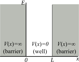
Figure 1:Particle in a box subject to infinitely high potential walls.
The Schrödinger equation for a particle in a box (PIB) is defined by a Hamiltonian operator that incorporates a potential energy which is infinitely large at the boundaries of the box and zero inside. This potential confines the particle within the box, where it can only possess kinetic energy.
The potential energy for PIB is defined:
The boundary conditions are:
The Hamiltonian operator in this case accounts only for kinetic energy:
Now, we have all the necessary ingredients to solve the time-independent Schrödinger equation for the 1D PIB:
Substituting the Hamiltonian, we get:
where is a positive real number that relates the particle’s energy to its wavefunction.
Solution and Boundary Conditions
Mathematically, the form of the 1D PIB problem is similar to the ordinary differential equation (ODE) used in the 1D vibrating guitar string problem. The key differences lie in the constant coefficients and the interpretation of the wavefunction.
The general solution to this differential equation is:
Applying the boundary condition , we find that , leaving us with:
Applying the boundary condition , we get:
This condition is satisfied when:
Thus, the wavefunction becomes:
Using the relationship , we can express the energy levels as:
The quantization of energy results from confining the wavefunction within a finite space. This is the reason bound states exhibit quantized energy levels. Atoms, molecules, and solids all possess discrete energy levels due to similar constraints.
This is the trial-energy experiment of the previous lecture in its simplest form. There the decaying tails admitted only special energies; here the walls do: reaches zero at only when a whole number of half-waves fits, .
Wavefunctions Must Be Normalized
Next, we determine the constant coefficient by enforcing the normalization condition:
To evaluate the integral, we use the trigonometric identity
Since the integral of over a full period from 0 to is zero, we are left with:
Solving for , we determine the normalization constant, which ensures that the square of the wavefunction integrates to 1.
PIB Eigenfunctions and Eigenvalues
Source
# synced: pib_ladder
import numpy as np
import matplotlib.pyplot as plt
from matplotlib.animation import FuncAnimation
from IPython.display import HTML
TEAL, CARDINAL, GRAY, PURPLE, ORANGE = "#107895", "#C8102E", "#6c757d", "#6a3d9a", "#e07b00"
plt.rcParams.update({"axes.spines.top": False, "axes.spines.right": False})
x = np.linspace(0, 1, 400)
fig, (ax1, ax2) = plt.subplots(1, 2, figsize=(8, 4.4), sharey=True, gridspec_kw={"wspace": 0.08})
for ax in (ax1, ax2):
ax.plot([0, 0, 1, 1], [18.3, 0, 0, 18.3], color="k", lw=2.6)
ax.set_xlim(-0.04, 1.04); ax.set_ylim(-0.4, 18.3)
ax.set_xticks([0, 0.5, 1]); ax.set_xticklabels(["0", "L/2", "L"]); ax.set_xlabel("x")
ax.spines["left"].set_visible(False)
for n in range(1, 5):
E, s = n * n, np.sin(n * np.pi * x)
for ax in (ax1, ax2):
ax.hlines(E, 0, 1, color=GRAY, lw=0.8, ls="--")
ax1.plot(x, E + 1.25 * s, color=TEAL, lw=2.4)
ax2.fill_between(x, E, E + 1.6 * s**2, color=CARDINAL, alpha=0.18, lw=0)
ax2.plot(x, E + 1.6 * s**2, color=CARDINAL, lw=2.2)
ax2.plot(np.arange(1, n) / n, np.full(n - 1, E), "o", color="k", ms=5, zorder=5)
ax2.text(1.06, E, rf"$n = {n}$, " + (r"$E_1$" if n == 1 else rf"${E}E_1$"), va="center", fontsize=11.5)
ax1.set_yticks([]); ax1.set_ylabel("energy")
ax1.set_title(r"$\psi_n(x)$, drawn on its level $E_n$", loc="left", fontsize=11)
ax2.set_title(r"$|\psi_n(x)|^2$: dots mark the $n-1$ nodes", loc="left", fontsize=11)
fig.subplots_adjust(left=0.05, right=0.83, top=0.92, bottom=0.12)
plt.show()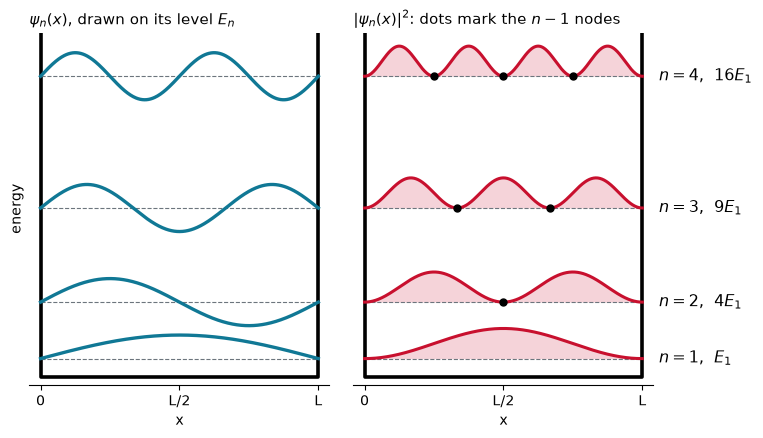
Fig. The four lowest states of the particle in a box, each drawn on its energy level . Left: the wavefunctions . Right: the probability densities ; the dots mark the nodes, where the particle is never found.
Discrete energy levels and zero point energy
Quantum particles are never at rest
The lowest energy an electron in a box can have is at , and it is not zero!
Keeping in mind that the energy is purely kinetic, this means a quantum particle never ceases its motion.
This is the uncertainty principle at work. Confining the particle to a length leaves a position spread in the ground state (Problem 2), and the momentum cannot be pinned down either: but , so . The product sits just above the Heisenberg limit . A smaller box means a larger and a larger kinetic energy.
The spacing of energy levels is finite and depends on the size of the box:
Increasing Box size leads to more classical behavior
As the box size is increased, the energy spacing gets smaller.
Thus quantum effects are more pronounced when an electron is bound in smaller regions of space.
Fig. Left: the three lowest levels of a particle in a box of length , each wavefunction drawn on its level. Right: the ground-state energy against box length. Shrinking the box raises every level as ; enlarging it lowers toward zero without ever reaching it. Energies in units of .
Non-uniform probabilities and nodes
Nodes imply zero probability to find an electron in the box.
at nodal points, which means zero probability.
This sharply contradicts classical mechanics, which bases its prediction on purely particle-like motion of the electron.
The existence of nodes implies a wave-like character of the electron.
There are nodes for quantum state
Recall that the sine function hits zero at integer multiples of : when
The wavefunction then has nodes at the points , , , ..., .
Note that we do not count the and points as nodes, because they are part of the boundary conditions that apply to all wavefunctions.
For instance, the nodes are at and .
For instance, the nodes are at , , and .
The dots in the right panel of the figure of the four lowest states mark these nodes.
Large quantum numbers: the classical box returns
As grows, the lobes of crowd together. A real detector has a finite resolution and averages over many lobes, and averages to over whole half-waves, so the measured density approaches the flat classical value .
Problem 1 gives the probability of catching the particle in the middle third of the box:
The correction to the classical dies off as . This is the correspondence principle: quantum predictions go over to classical ones at large quantum numbers. A 1 g marble crawling at 1 cm/s across a 30 cm box has , far beyond any lobe we could resolve.
Fig. The probability density of state against the flat classical density . The shaded band is the middle third of the box; its probability tends to the classical as grows.
Superposition: the particle sloshes
A single state is stationary. Its phase turns, but the time factor has absolute value one, so never changes (see the phase clocks in the previous lecture).
A superposition of two states does move. Take equal amounts of the two lowest states:
Multiplying by the complex conjugate (Problem 2 of the previous lecture) leaves a fixed part and a cross term that oscillates at the difference of the two phase rates, :
Source
# synced: box_slosh
import numpy as np
import matplotlib.pyplot as plt
from matplotlib.animation import FuncAnimation
from IPython.display import HTML
TEAL, CARDINAL, GRAY, PURPLE, ORANGE = "#107895", "#C8102E", "#6c757d", "#6a3d9a", "#e07b00"
plt.rcParams.update({"axes.spines.top": False, "axes.spines.right": False})
x = np.linspace(0, 1, 400)
p1, p2 = np.sqrt(2) * np.sin(np.pi * x), np.sqrt(2) * np.sin(2 * np.pi * x)
fixed, cross = 0.5 * (p1**2 + p2**2), p1 * p2 # |Psi|^2 = fixed + cross cos(wt): even + odd about L/2
nf = 60
ts = np.linspace(0, 2 * np.pi, nf, endpoint=False) # E1 = 1, E2 = 4, hbar = 1: w = 3, three sloshes
xbar = lambda t: 0.5 - 16 / (9 * np.pi**2) * np.cos(3 * t) # <x>(t) = L/2 + x12 cos(wt), x12 = -16L/9pi^2
th = np.linspace(0, 2 * np.pi, 200)
fig = plt.figure(figsize=(7.2, 3.4))
gs = fig.add_gridspec(2, 2, width_ratios=[2.3, 1], height_ratios=[2, 1], hspace=0.42, wspace=0.08)
ax, axx = fig.add_subplot(gs[0, 0]), fig.add_subplot(gs[1, 0])
axc, axl = fig.add_subplot(gs[0, 1]), fig.add_subplot(gs[1, 1])
ax.plot(x, fixed, color=GRAY, lw=1.8, ls="--", label=r"$\frac{1}{2}(\psi_1^2 + \psi_2^2)$")
(dens,) = ax.plot([], [], color=CARDINAL, lw=2.8, label=r"$|\Psi|^2$")
band = [ax.fill_between(x, 0 * x, color=CARDINAL, alpha=0.18, lw=0)]
(mark,) = ax.plot([], [], marker="^", color=PURPLE, ms=14, zorder=6, ls="none", label=r"$\langle x\rangle$")
ax.plot([0, 0, 1, 1], [3.35, 0, 0, 3.35], color="k", lw=2.6) # peak of |Psi|^2 is 3.10
ax.set_xlim(-0.02, 1.02); ax.set_ylim(0, 3.35); ax.set_xticks([]); ax.set_yticks([])
ax.spines["left"].set_visible(False); ax.spines["bottom"].set_visible(False)
ax.legend(loc="lower left", bbox_to_anchor=(0, 0.97), ncol=3, frameon=False, fontsize=13,
handlelength=1.6, columnspacing=1.4)
axx.axhline(0, color=GRAY, lw=0.8)
(crs,) = axx.plot([], [], color=PURPLE, lw=2.6)
cband = [axx.fill_between(x, 0 * x, color=PURPLE, alpha=0.18, lw=0)]
axx.set_xlim(-0.02, 1.02); axx.set_ylim(-1.7, 1.7); axx.set_yticks([])
axx.set_xticks([0, 0.5, 1]); axx.set_xticklabels(["0", "L/2", "L"], fontsize=13)
axx.spines["left"].set_visible(False)
axx.set_title(r"cross term $\psi_1\psi_2\cos\omega t$", loc="left", fontsize=13, color=PURPLE)
for a in (ax, axx):
a.axvline(0.5, color=GRAY, lw=0.8, ls=":")
axc.plot(np.cos(th), np.sin(th), color=GRAY, lw=1, ls="--")
(arc,) = axc.plot([], [], color=PURPLE, lw=3.2, label=r"$\omega t$")
(h1,) = axc.plot([], [], color=TEAL, lw=3.2, label=r"$E_1$")
(h2,) = axc.plot([], [], color=ORANGE, lw=3.2, label=r"$E_2 = 4E_1$")
axc.set_aspect("equal"); axc.set_xlim(-1.15, 1.15); axc.set_ylim(-1.15, 1.15); axc.set_axis_off()
axc.set_title("phase clocks", fontsize=13)
axl.set_axis_off()
axl.legend(handles=[h1, h2, arc], loc="center", frameon=False, fontsize=13, handlelength=1.2)
fig.subplots_adjust(left=0.02, right=0.99, top=0.87, bottom=0.1)
def update(i):
t = ts[i]
c = cross * np.cos(3 * t)
dens.set_data(x, fixed + c)
band[0].remove(); band[0] = ax.fill_between(x, fixed + c, color=CARDINAL, alpha=0.18, lw=0)
mark.set_data([xbar(t)], [0.14])
crs.set_data(x, c)
cband[0].remove(); cband[0] = axx.fill_between(x, c, color=PURPLE, alpha=0.18, lw=0)
a1, a2 = -t, -4 * t # clock hands: e^{-iE1 t}, e^{-iE2 t}
d = (a1 - a2) % (2 * np.pi) # angle between the hands, w t
s = np.linspace(a2, a2 + d, 40) if d <= np.pi else np.linspace(a1, a1 + 2 * np.pi - d, 40)
arc.set_data(0.42 * np.cos(s), 0.42 * np.sin(s))
h1.set_data([0, np.cos(a1)], [0, np.sin(a1)]); h2.set_data([0, np.cos(a2)], [0, np.sin(a2)])
ani = FuncAnimation(fig, update, frames=nf, interval=90, blit=False)
plt.close(fig)
HTML(ani.to_jshtml())Fig. An equal superposition of and . Top: the density is the fixed part (dashed) plus the cross term; the triangle marks . Bottom: the cross term . Right: the phase clocks of the two states; the angle between their hands is .
The fixed part is symmetric about the center of the box, so on its own it balances at . The cross term is odd about the center: it adds probability on one side, removes the same amount on the other, and flips sign every half period. The mean position swings with it:
For an electron, an oscillating is an oscillating electric dipole: a tiny antenna that emits or absorbs light of angular frequency , that is photons with . This is the link to the colors of conjugated molecules in the applications below. The general theory is in Time Dependence.
Quantum PIB in 3D
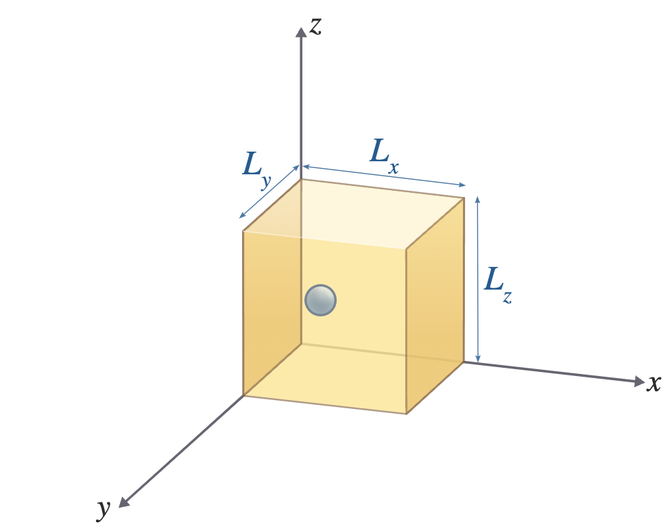
Figure 2:Particle in a 3D box subject to infinitely high potential walls.
Where we set for particle inside the box and enforce the solutions to be normalized within the confines of the box (electron must be somewhere in the box!)
Consider a particle in a box with side lengths in , in , and in . The potential is zero inside the box and infinite outside it. Again, the potential term can be handled by boundary conditions (i.e., infinite potential implies that the wavefunction must be zero there). The above equation can now be written as:
Note the Laplacian symbol , which concisely denotes the sum of the three second-order derivatives with respect to the spatial variables. We will see this operator in all 3D problems.
In general, when the potential term can be expressed as a sum of terms that depend separately on , , and , the solutions can be written as a product:
By substituting and dividing by , we obtain:
The total energy consists of a sum of three terms, each depending separately on , , and . Thus we can write and separate the equation into three one-dimensional problems:
Thus we find energy quantization due to spatial confinement of the quantum wave function in the , , and dimensions:
Energy is quantized and when , we find that the energy levels can also be degenerate (i.e., the same energy with different values of and ).
In most cases, degeneracy in quantum mechanics arises from symmetry. When , the first excited level is triply degenerate: , and are one shape turned to face different axes. When only , that level splits into a pair and a single state; the pair lies lower when is shorter than .
Table of energy levels for a cubic box
Energies in units of , so . The degeneracy counts the states on each level.
| states | degeneracy | |
|---|---|---|
| 3 | (1,1,1) | 1 |
| 6 | (2,1,1), (1,2,1), (1,1,2) | 3 |
| 9 | (2,2,1), (2,1,2), (1,2,2) | 3 |
| 11 | (3,1,1), (1,3,1), (1,1,3) | 3 |
| 12 | (2,2,2) | 1 |
| 14 | all six orderings of (3,2,1) | 6 |
| 17 | (3,2,2), (2,3,2), (2,2,3) | 3 |
| 18 | (4,1,1), (1,4,1), (1,1,4) | 3 |
| 19 | (3,3,1), (3,1,3), (1,3,3) | 3 |
| 21 | all six orderings of (4,2,1) | 6 |
| 22 | (3,3,2), (3,2,3), (2,3,3) | 3 |
| 24 | (4,2,2), (2,4,2), (2,2,4) | 3 |
| 26 | all six orderings of (4,3,1) | 6 |
| 27 | (3,3,3) and the three orderings of (5,1,1) | 4 |
The last row is an accidental degeneracy: , and no rotation of the cube turns into .
Fig. Surfaces of constant in a cubic box, red and blue for the two signs. Set and then : the same shape turned by , so the two states share an energy.
The level diagram below does the counting. Each short bar is one state. With all three sides equal, states related by a rotation of the box share a level; stretch or squeeze one side and those levels split.
Fig. The seven lowest levels of a particle in a rectangular box. Each bar is one state and counts the states on a level. A cube has levels with ; changing one side breaks the symmetry and splits them.
Note on Computing Average Properties from a Wave Function
Because of the probabilistic interpretation of the wave function, average properties can be computed from the wave function. The general formula is
where is any operator. This could be momentum, kinetic energy, and so on. Below are a few problems illustrating how to do such calculations.
To calculate the average position (or expectation value of position) for a particle in a 1D box, follow the steps shown in the example below.
Example: Calculate average (expectation) of position,
1. Wavefunction of the Particle in a 1D Box
The wavefunction for a particle in a 1D box of length with infinite potential walls at and is given by:
where:
is the quantum number (1, 2, 3, ...),
is the length of the box,
is the wavefunction.
2. Expectation Value of Position
The expectation value of the position for a particle is given by:
This integral gives the average position of the particle based on the probability density . For the wavefunction , the probability density is:
3. Set Up the Integral
Substitute into the expression for :
This is the integral you need to solve to find the average position.
4. Solve the Integral
The integral can be simplified using known trigonometric identities. First, use the identity:
So, the integral becomes:
Simplifying:
Now split this into two integrals:
5. Evaluate the Integrals
The first integral is straightforward:
The second integral can be solved using integration by parts or by referring to standard integral tables. It turns out that this integral evaluates to 0 for any integer . Thus:
6. Final Result
Thus, the expectation value of position simplifies to:
7. Interpretation
For any quantum state , the average position of a particle in a 1D box is always:
This result makes sense intuitively because, due to the symmetry of the problem, the particle is equally likely to be found on either side of the box, so its average position is right in the middle of the box at .
Summary
To find the average position of a particle in a 1D box for a general wavefunction:
Use the wavefunction ,
Set up the expectation value integral ,
Solve the integral, which results in for all .
Thus, the particle’s average position is always at the midpoint of the box, independent of the quantum number .
Applications: electronic transitions in conjugated molecules
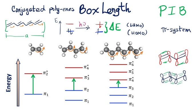
One of the most useful applications of the particle in a box is estimating the color of light absorbed by π-conjugated molecules. In molecules with alternating single and double bonds, the π-electrons are delocalized over the conjugated region and behave, to a first approximation, like particles confined to a box whose length is the length of the conjugated chain.
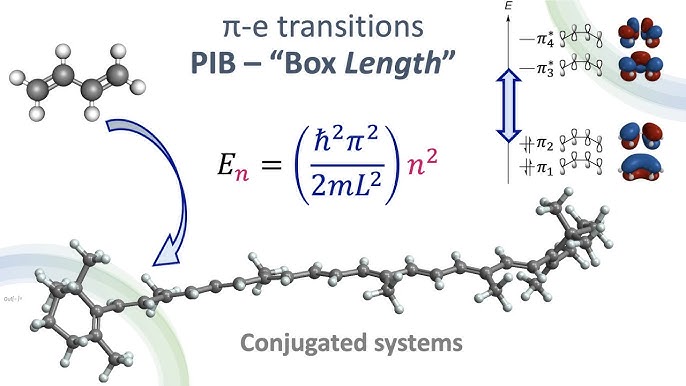
A linear conjugated system (a polyene) modeled as a 1D particle in a box: the delocalized π-electrons are confined to the length of the conjugated chain.
1D box models linear conjugated systems such as butadiene and longer polyenes. The box length is the length of the conjugated chain, and the level spacing sets the wavelength of light absorbed.
2D box models π-electrons delocalized over a two-dimensional region, such as aromatic rings or graphene fragments.
Aromatic and extended π-systems modeled as a 2D particle in a box.
Worked example: butadiene
Consider butadiene (C₄H₆), whose four π-electrons are delocalized over the conjugated chain. We estimate the wavelength that excites one π-electron across the gap.
Step 1: length of the box. Butadiene, CH₂=CH-CH=CH₂, has two C=C bonds and one C-C bond between its end carbons (C=C ≈ 1.35 Å, C-C ≈ 1.54 Å):
Step 2: fill the levels. Each level holds two electrons (Pauli), so the four π-electrons fill and . The highest occupied level is and the lowest empty one is , so the absorption is the transition.
Step 3: transition energy and wavelength. With , the absorbed photon satisfies
Source
import numpy as np
h = 6.626e-34 # Planck constant (J s)
m = 9.109e-31 # electron mass (kg)
c = 3.0e8 # speed of light (m/s)
# box ending at the end carbons, then one carbon radius (0.77 A) past each end
for label, L in [("L = 4.24 A", 4.24e-10), ("L = 5.78 A", 5.78e-10)]:
E = lambda n: n**2 * h**2 / (8 * m * L**2)
dE = E(3) - E(2) # HOMO (n=2) -> LUMO (n=3)
lam = h * c / dE
print(f"{label}: Delta E (2 -> 3) = {dE:.3e} J, absorption wavelength = {lam * 1e9:.0f} nm")L = 4.24 A: Delta E (2 -> 3) = 1.676e-18 J, absorption wavelength = 119 nm
L = 5.78 A: Delta E (2 -> 3) = 9.017e-19 J, absorption wavelength = 220 nm
With the box ending at the end carbons, the estimate (about 119 nm) lands deep in the ultraviolet, well short of the measured 217 nm. The π-electrons do not stop at the end carbons, though: extending the box by one carbon radius (0.77 Å) past each end gives Å and about 220 nm, close to experiment. The simple model captures the key trend: longer conjugation means a longer box, smaller level spacing, and absorption shifted toward the red, which is why extended π-systems like carotenes are colored.
Problems
Problem 1: Compute probability of finding particle somewhere
Compute the probability of observing the particle in a box in the domain .
Solution
Since the square of the wave function is a probability density, we can determine the probability of observing the particle in a particular domain using the relationship
We simply use the above equation together with the normalized particle-in-a-box wave function:
We will use the definite integral of from a table:
Perform a -substitution on the integral above to put it into the table form:
Problem 2: Compute an expectation of 
Compute the average of for a particle in a box.
Solution
To compute the average value of , we start by writing the integral expression:
For the particle in a box, we can limit the domain, and thus the bounds of integration, to . We can also set .
Thus, for a particle in a 1D box of size , we get
From an integral table we find that
We use this equation with and get:
This result, combined with the result for , can be used to determine , the standard deviation of the particle’s position:
Problem 3: Compute expectation of energy
Compute the average energy of a particle in a box.
Solution
The average energy of the particle in a box is a special case of computing an average quantity. We start by writing out the standard definition of an average computed from a wavefunction:
where is the total energy operator. We know the total energy operator by another symbol, namely . We plug this into the above equation to get:
We now recognize that the particle-in-a-box wavefunctions we are discussing were derived from the Schrödinger equation:
where is a scalar. Thus, for the average energy we get:
The last equality holds because the wave functions are normalized.
Problem 4: Compute expectation of momentum
Compute the average momentum for a particle in a box.
Solution
To compute the average momentum of a particle in a 1D box, we start in the usual way:
Recall that the momentum operator in one dimension is given by
We now substitute this into the above equation and solve:
where the last equality can be found in an integral table.
So the average momentum of a particle in a box is zero. This is because it is equally probable for the particle to be moving forward and backward.
Problem 5
Consider an electron in superfluid helium (He) where it forms a solvation cavity with a radius of . Calculate the zero-point energy and the energy difference between the ground and first excited states by approximating the electron by a particle in a 3-dimensional box.
Solution
Problem 6: Energy Levels in a 3D Box
A particle is confined in a 3D box with side lengths . The energy levels for a particle in this box are given by the formula:
where , , are the quantum numbers associated with the particle’s motion in the -, -, and -directions.
Calculate the energy levels for the quantum states with , , and , , . Are these energy levels degenerate?
Solution
Problem 7: Degeneracy of Energy Levels
Consider a particle confined in a cubic box with side lengths . The energy levels are given by the same formula as in Problem 6.
Part 1: Find the degeneracy of the energy level corresponding to the quantum number sum .
Part 2: Write down all the quantum number triplets that correspond to this energy level.
Solution
Part 1: We want to find the quantum numbers that satisfy:
We can check different combinations of , , and :
For , , and :
Other permutations of these quantum numbers will give the same energy:
Part 2: The energy level corresponding to has 6 degenerate states, since the quantum number triplets are , , , , , and .
Problem 8: Degeneracy of the Ground State
Part 1: What is the degeneracy of the ground state (the lowest energy state) for a particle in a cubic box?
Part 2: Explain why the ground state does not have degeneracy.
Solution
Part 1: The ground state corresponds to the quantum numbers . The energy for this state is:
There is only one combination of quantum numbers that gives this energy, so the degeneracy of the ground state is 1.
Part 2: The ground state is non-degenerate because there is only one way to assign the quantum numbers . Degeneracy arises when multiple different sets of quantum numbers give the same energy, which is not the case for the ground state.
Problem 9: Higher Energy Degeneracy
Consider a particle in a cubic box. The energy levels are quantized as:
Part 1: Find the quantum numbers that give the same energy for the quantum number sum . How many degenerate states correspond to this energy?
Part 2: What is the degeneracy of this energy level?
Solution
Part 1: We want to solve:
Possible combinations of , , and :
, , gives .
Permutations of are:
also gives 9, but it is not allowed: each quantum number is at least 1, since makes .
Part 2: The degeneracy for the energy level corresponding to is 3: the three permutations of .
Problem 10: Absorption of a conjugated diene
A conjugated diene has a conjugation length of 5 Å. Using the 1D particle in a box, calculate the wavelength absorbed when a π-electron is excited from to . Use and .
Solution
Problem 11: Total conjugation length of a polyene
A polyene has 6 alternating bonds with Å and Å. Find the total conjugation length and the wavelength needed to excite a π-electron from to .
Solution
Then and .
Problem 12: A higher transition
A linear conjugated molecule has 8 alternating C-C bonds (1.40 Å single, 1.35 Å double). Calculate the wavelength absorbed for the transition.
Problem 13: Triene transition
A conjugated triene has a conjugation length of 7.5 Å. Find the wavelength absorbed for the transition.
Solution
Problem 14: A transition between excited states
A polyene of 10 carbons has Å and Å. Find the total conjugation length and the wavelength for the transition.
Problem 15: A 2D box for a graphene fragment
Model the π-electrons of a graphene-like fragment as a 2D particle in a box with and . Calculate the energy of the state , .