Time Dependence - Quantum Mechanics for Chemistry

What you need to know

Every state evolves by one recipe: expand it in energy eigenstates, attach to each the phase $e^{-iE_nt/\hbar}$ of its own clock, and add the pieces back up. Diagonalize $\hat{H}$ once, and the motion of any starting state follows.
The energy probabilities $\lvert c_n\rvert^2$ never change, so neither do $\langle E\rangle$ , $\sigma_E$ or the normalization. Only the relative phases change, and every kind of motion comes from them.
An average changes as $\frac{d}{dt}\langle A\rangle = \frac{i}{\hbar}\langle[\hat{H},\hat{A}]\rangle$ : observables that commute with $\hat{H}$ are constants of motion, such as the energy, and the momentum of a free particle.
Ehrenfest’s theorem: averages obey Newton’s laws, $d\langle x\rangle/dt = \langle p\rangle/m$ and $d\langle p\rangle/dt = -\langle dV/dx\rangle$ . In a harmonic well a packet moves exactly like the classical particle; in other wells it spreads and falls behind.
Motion contains only energy differences, the Bohr frequencies $(E_n - E_m)/\hbar$ that spectroscopy measures. When those differences are commensurate, all the clocks realign and the state revives.

Operators 1, Operators 2 and Measurement described a single instant. This lecture adds time, the last postulate: the state evolves by the time-dependent Schrödinger equation, $i\hbar\,\partial\Psi/\partial t = \hat{H}\Psi$ .

One recipe for all motion¶

A stationary state $\psi_n(x)\,e^{-iE_nt/\hbar}$ solves the time-dependent equation on its own: its phase turns at the rate $E_n/\hbar$ and its density never moves (the phase clocks of The Schrödinger Equation).
The equation is linear, so any sum of stationary states is also a solution, with each term keeping its own clock. Since the energy eigenstates form a complete basis, every starting state is such a sum.

Check: the sum solves the time-dependent Schrödinger equation

Differentiate each term in time, then compare with $\hat{H}$ acting on each term, using $\hat{H}\psi_n = E_n\psi_n$ :

i\hbar\,\frac{\partial\Psi}{\partial t} = \sum_n c_n\,i\hbar\left(-\frac{iE_n}{\hbar}\right)e^{-iE_nt/\hbar}\,\psi_n = \sum_n c_n\,E_n\,e^{-iE_nt/\hbar}\,\psi_n

(2)

\hat{H}\Psi = \sum_n c_n\,e^{-iE_nt/\hbar}\,\hat{H}\psi_n = \sum_n c_n\,E_n\,e^{-iE_nt/\hbar}\,\psi_n

(3)

The two sides agree term by term. At $t = 0$ every phase is 1, so the sum starts from the right state.

We have already met the simplest cases. One term: nothing moves. Two terms: the density sloshes at $(E_2 - E_1)/\hbar$ , as in Particle in a Box, and the ammonia molecule of Tunneling flips back and forth. Here are three terms, the superposition $\frac{1}{2}\psi_1 + \frac{1}{2}\psi_2 + \frac{1}{\sqrt{2}}\psi_3$ whose energy readings we simulated in Measurement:

# synced: evolve_recipe
import numpy as np
import matplotlib.pyplot as plt
from matplotlib.animation import FuncAnimation
from IPython.display import HTML

TEAL, CARDINAL, GRAY, PURPLE, ORANGE = "#107895", "#C8102E", "#6c757d", "#6a3d9a", "#e07b00"
plt.rcParams.update({"axes.spines.top": False, "axes.spines.right": False})
x = np.linspace(0, 1, 400)                                  # box, L = hbar = 1, E_n = n^2 E1 with E1 = 1
c = np.array([0.5, 0.5, np.sqrt(0.5)])                      # the state of the Measurement lecture
ns = np.array([1, 2, 3])
phis = np.sqrt(2) * np.sin(np.outer(ns, np.pi * x))
nf = 44
ts = np.linspace(0, 2 * np.pi, nf, endpoint=False)          # one full period T = 2 pi hbar / E1
tt = np.linspace(0, 2 * np.pi, 500)
amp = lambda t: (c * np.exp(-1j * ns**2 * t)) @ phis
xbar = np.array([np.trapezoid(x * np.abs(amp(t))**2, x) for t in tt])
th = np.linspace(0, 2 * np.pi, 200)
fig = plt.figure(figsize=(8.4, 4.4))
gs = fig.add_gridspec(3, 2, width_ratios=[2.5, 1], height_ratios=[1, 1, 1], hspace=0.55, wspace=0.12)
ax = fig.add_subplot(gs[0:2, 0]); axx = fig.add_subplot(gs[2, 0])
(dens,) = ax.plot([], [], color=CARDINAL, lw=2.6)
band = [ax.fill_between(x, 0 * x, color=CARDINAL, alpha=0.16, lw=0)]
(mark,) = ax.plot([], [], marker="^", color=PURPLE, ms=13, ls="none", zorder=6)
ax.plot([0, 0, 1, 1], [5.4, 0, 0, 5.4], color="k", lw=2.6)
ax.set_xlim(-0.02, 1.02); ax.set_ylim(0, 5.4); ax.set_xticks([]); ax.set_yticks([])
ax.spines["left"].set_visible(False); ax.spines["bottom"].set_visible(False)
axx.plot(tt / (2 * np.pi), xbar, color=PURPLE, lw=1, alpha=0.25)
(trace,) = axx.plot([], [], color=PURPLE, lw=2.4); (dot,) = axx.plot([], [], "o", color=PURPLE, ms=7)
axx.axhline(0.5, color=GRAY, lw=0.8, ls=":")
axx.set_xlim(0, 1); axx.set_ylim(0.2, 0.8); axx.set_yticks([0.25, 0.5, 0.75]); axx.set_yticklabels(["L/4", "L/2", "3L/4"])
axx.set_xticks([0, 0.25, 0.5, 0.75, 1]); axx.set_xticklabels(["0", "T/4", "T/2", "3T/4", "T"])
axx.tick_params(labelsize=11); axx.set_title(r"$\langle x\rangle(t)$", loc="left", fontsize=12.5, color=PURPLE)
hands = []
for r, (n, cn, col) in enumerate(zip(ns, c, (TEAL, ORANGE, CARDINAL))):
    axc = fig.add_subplot(gs[r, 1])
    axc.plot(np.cos(th), np.sin(th), color=GRAY, lw=0.8, ls="--")
    (hd,) = axc.plot([], [], color=col, lw=3.2); (tp,) = axc.plot([], [], "o", color=col, ms=6)
    axc.set_aspect("equal"); axc.set_xlim(-1.1, 1.1); axc.set_ylim(-1.1, 1.1); axc.axis("off")
    axc.text(1.25, 0, rf"$n = {n}$" + "\n" + rf"$|c_{n}|^2 = {cn**2:.2f}$" + "\n" + (r"$E_1$" if n == 1 else rf"${n * n}E_1$"),
             fontsize=11, va="center", color=col)
    hands.append((hd, tp, n, cn / c.max()))
fig.subplots_adjust(left=0.08, right=0.9, top=0.93, bottom=0.08)

def update(i):
    t = ts[i]
    d = np.abs(amp(t))**2
    dens.set_data(x, d)
    band[0].remove(); band[0] = ax.fill_between(x, d, color=CARDINAL, alpha=0.16, lw=0)
    xm = np.trapezoid(x * d, x)
    mark.set_data([xm], [0.25])
    k = int(round(t / (2 * np.pi) * (len(tt) - 1)))
    trace.set_data(tt[:k + 1] / (2 * np.pi), xbar[:k + 1]); dot.set_data([t / (2 * np.pi)], [xm])
    for hd, tp, n, ln in hands:
        z = ln * np.exp(-1j * n * n * t)
        hd.set_data([0, z.real], [0, z.imag]); tp.set_data([z.real], [z.imag])
    ax.set_title(rf"$|\Psi(x,t)|^2$ at $t = {t / (2 * np.pi):.2f}\,T$   (" + "\u25b2" + r" marks $\langle x\rangle$)", loc="left", fontsize=12.5)

ani = FuncAnimation(fig, update, frames=nf, interval=110, blit=False)
plt.close(fig)
HTML(ani.to_jshtml())

Fig. Three box states, each with a clock that turns at its own rate, $E_n/\hbar = E_1/\hbar$ , $4E_1/\hbar$ and $9E_1/\hbar$ . The length of each hand, $\lvert c_n\rvert$ , never changes; only the angles between the hands do. Their interference moves the density (top) and its average position (bottom). After $T = 2\pi\hbar/E_1$ every hand is back where it started, and so is the state.

On a grid, the recipe is three lines of numpy once $\hat{H}$ is a matrix: diagonalize, project the starting state onto the eigenvectors, and attach the phases. Here a packet shaped like the ground state of a particle on a spring starts displaced to $x = 3$ ( $\hbar = m = \omega = 1$ ):

import numpy as np

N = 600
x = np.linspace(-10, 10, N); dx = x[1] - x[0]
H = -0.5 * (np.eye(N, k=1) - 2 * np.eye(N) + np.eye(N, k=-1)) / dx**2 + np.diag(0.5 * x**2)
E, phi = np.linalg.eigh(H)                    # 1. diagonalize once
phi = phi / np.sqrt(dx)                       #    columns normalized as functions

psi0 = np.exp(-(x - 3)**2 / 2) / np.pi**0.25  # ground-state shape, displaced to x = 3
c = phi.T @ psi0 * dx                         # 2. expand: c_n = <phi_n|psi0>

for t in [0, np.pi / 2, np.pi, 2 * np.pi]:
    psi_t = phi @ (c * np.exp(-1j * E * t))   # 3. attach the phases and add up
    rho = np.abs(psi_t)**2
    print(f"t = {t:4.2f}   norm = {np.sum(rho) * dx:.6f}   <x> = {np.sum(x * rho) * dx:+.3f}   3 cos t = {3 * np.cos(t):+.3f}")

t = 0.00   norm = 1.000000   <x> = +3.000   3 cos t = +3.000
t = 1.57   norm = 1.000000   <x> = +0.004   3 cos t = +0.000
t = 3.14   norm = 1.000000   <x> = -3.000   3 cos t = -3.000
t = 6.28   norm = 1.000000   <x> = +3.000   3 cos t = +3.000

The norm stays exactly 1, and the average position follows $3\cos t$ , the motion of a classical mass on a spring released from $x = 3$ . Both facts are explained below.
The translation table of Operators 1 gets its last row:

	integral	Dirac	numpy on a grid
time evolution	$\sum_n c_n e^{-iE_nt/\hbar}\psi_n(x)$	$e^{-i\hat{H}t/\hbar}\lvert\Psi(0)\rangle$	`phi @ (c * np.exp(-1j * E * t / hbar))`

What never changes¶

Each coefficient only turns: $\lvert c_n e^{-iE_nt/\hbar}\rvert^2 = \lvert c_n\rvert^2$ . So the probabilities of the energy readings are frozen, and with them $\langle E\rangle$ and $\sigma_E$ . An energy measurement at any time gives the same statistics as at $t = 0$ .
The normalization is conserved too. The cross terms vanish by orthogonality at every instant:

\langle \Psi(t) \vert \Psi(t) \rangle = \sum_m\sum_n c_m^*\,c_n\,e^{i(E_m - E_n)t/\hbar}\,\langle \psi_m \vert \psi_n \rangle = \sum_n \lvert c_n\rvert^2 = 1

(4)

In the language of Operators as Matrices, the evolution operator $e^{-i\hat{H}t/\hbar}$ is unitary: it rotates the state vector without changing its length. The particle is always somewhere.
What does change are the relative phases between the coefficients. They control the interference terms, and so the shape of $\lvert\Psi(x,t)\rvert^2$ , the average position, and anything else that does not commute with $\hat{H}$ .

Constants of motion¶

How fast does an average change? Differentiate $\langle A\rangle = \langle \Psi \vert \hat{A} \vert \Psi \rangle$ with the product rule, and replace the time derivatives using the Schrödinger equation, $\partial_t\lvert\Psi\rangle = \hat{H}\lvert\Psi\rangle/i\hbar$ and $\partial_t\langle\Psi\rvert = -\langle\Psi\rvert\hat{H}/i\hbar$ :

\frac{d}{dt}\langle A\rangle = -\frac{1}{i\hbar}\langle \Psi \vert \hat{H}\hat{A} \vert \Psi \rangle + \frac{1}{i\hbar}\langle \Psi \vert \hat{A}\hat{H} \vert \Psi \rangle + \Big\langle \frac{\partial \hat{A}}{\partial t}\Big\rangle

(5)

For an operator with no explicit time dependence, the average is constant whenever $\hat{A}$ commutes with $\hat{H}$ . Such observables are constants of motion, and the commutators of Operators 2 tell us which ones they are:

observable	commutator with $\hat{H} = \hat{p}^2/2m + V(x)$	conserved when
energy $\hat{H}$	$[\hat{H},\hat{H}] = 0$	always
momentum $\hat{p}$	$[\hat{H},\hat{p}] = i\hbar\,dV/dx$	no force, $V$ constant
parity $\hat{\Pi}$	$[\hat{H},\hat{\Pi}] = 0$ if $V(-x) = V(x)$	the potential is symmetric
position $\hat{x}$	$[\hat{H},\hat{x}] = -i\hbar\,\hat{p}/m$	only while $\langle p\rangle$ stays zero

The free particle shows the difference at a glance. Its momentum commutes with $\hat{H}$ ; its position does not:

# synced: free_spread
import numpy as np
import matplotlib.pyplot as plt
from matplotlib.animation import FuncAnimation
from IPython.display import HTML

TEAL, CARDINAL, GRAY, PURPLE, ORANGE = "#107895", "#C8102E", "#6c757d", "#6a3d9a", "#e07b00"
plt.rcParams.update({"axes.spines.top": False, "axes.spines.right": False})
x = np.linspace(-25, 45, 2048, endpoint=False); dx = x[1] - x[0]   # hbar = m = 1
k = 2 * np.pi * np.fft.fftfreq(x.size, d=dx)
s0, k0 = 0.8, 2.5                                           # |psi|^2 starts with width s0 and moves at speed k0
psi0 = np.exp(-x**2 / (4 * s0**2) + 1j * k0 * x); psi0 = psi0 / np.sqrt(np.sum(np.abs(psi0)**2) * dx)
f0 = np.fft.fft(psi0)
nf = 36
ts = np.linspace(0, 7, nf)
p = np.linspace(-0.5, 5.5, 400)
php = np.exp(-(p - k0)**2 * 2 * s0**2); php = php / np.trapezoid(php, p)
fig, (ax, axp) = plt.subplots(2, 1, figsize=(8, 4.2), gridspec_kw={"height_ratios": [1.6, 1], "hspace": 0.6})
(lx,) = ax.plot([], [], color=TEAL, lw=2.4); bx = [ax.fill_between(x, 0 * x, color=TEAL, alpha=0.2, lw=0)]
(cl,) = ax.plot([], [], "o", color=PURPLE, ms=9, zorder=5, label=r"classical particle, $x = p_0t/m$")
ax.set_xlim(-6, 22); ax.set_ylim(0, 0.56); ax.set_yticks([]); ax.spines["left"].set_visible(False)
ax.set_xlabel(r"position $x$", fontsize=12); ax.tick_params(labelsize=11)
ax.legend(loc="upper right", frameon=False, fontsize=11.5)
axp.fill_between(p, php, color=CARDINAL, alpha=0.2, lw=0); axp.plot(p, php, color=CARDINAL, lw=2.4)
axp.set_xlim(-0.5, 5.5); axp.set_yticks([]); axp.spines["left"].set_visible(False)
axp.set_xlabel(r"momentum $p$", fontsize=12); axp.tick_params(labelsize=11)
axp.set_title(r"$|\phi(p)|^2$: the same at every $t$, because $[\hat{p},\hat{H}] = 0$", loc="left", fontsize=12.5)
fig.subplots_adjust(left=0.03, right=0.98, top=0.9, bottom=0.13)

def update(i):
    t = ts[i]
    d = np.abs(np.fft.ifft(f0 * np.exp(-0.5j * k**2 * t)))**2
    lx.set_data(x, d); bx[0].remove(); bx[0] = ax.fill_between(x, d, color=TEAL, alpha=0.2, lw=0)
    cl.set_data([k0 * t], [0.02])
    sx = s0 * np.sqrt(1 + (t / (2 * s0**2))**2)
    ax.set_title(rf"$|\Psi(x,t)|^2$ at $t = {t:.1f}$:  $\Delta x = {sx:.2f}$ grows,  $\Delta p = {1 / (2 * s0):.2f}$ stays",
                 loc="left", fontsize=12.5)

ani = FuncAnimation(fig, update, frames=nf, interval=120, blit=False)
plt.close(fig)
HTML(ani.to_jshtml())

Fig. A free Gaussian packet. Top: the position density moves at the classical speed (dot) and spreads, because its momentum components travel at different speeds. Bottom: the momentum distribution is the same at every instant, because $[\hat{p},\hat{H}] = 0$ : every $\lvert c_p\rvert^2$ is frozen, exactly like the $\lvert c_n\rvert^2$ of a bound state.

Ehrenfest’s theorem: averages obey Newton¶

Apply the rule for averages to $\hat{x}$ and $\hat{p}$ , using the commutators in the table: $\frac{i}{\hbar}\big(-i\hbar\langle p\rangle/m\big) = \langle p\rangle/m$ and $\frac{i}{\hbar}\,i\hbar\,\langle dV/dx\rangle = -\langle dV/dx\rangle$ .

These are Newton’s equations, with averages. But the force on the packet is the force averaged over the packet, $-\langle dV/dx\rangle$ , not the force at its center, $-V'(\langle x\rangle)$ . The two agree only when the force is linear in $x$ : a uniform field or a harmonic well. There the center of the packet follows the classical trajectory exactly, whatever the packet’s shape. In any other well the parts of the packet feel different forces, the packet spreads, and its center falls behind:

# synced: ehrenfest_wells
import numpy as np
import matplotlib.pyplot as plt
from matplotlib.animation import FuncAnimation
from IPython.display import HTML

TEAL, CARDINAL, GRAY, PURPLE, ORANGE = "#107895", "#C8102E", "#6c757d", "#6a3d9a", "#e07b00"
plt.rcParams.update({"axes.spines.top": False, "axes.spines.right": False})
x = np.linspace(-6, 6, 600); dx = x[1] - x[0]              # hbar = m = 1, both packets start at rest at x0
x0 = -2.5
T = -0.5 * (np.eye(x.size, k=1) - 2 * np.eye(x.size) + np.eye(x.size, k=-1)) / dx**2
psi0 = np.exp(-(x - x0)**2 / 2) / np.pi**0.25
nf, tmax = 44, 9.4
ts = np.linspace(0, tmax, nf)
wells = [(0.5 * x**2, lambda y: y, lambda y: 0.5 * y**2, r"harmonic, $V = \frac{1}{2}x^2$", TEAL),
         (0.1 * x**4, lambda y: 0.4 * y**3, lambda y: 0.1 * y**4, r"quartic, $V = 0.1\,x^4$", ORANGE)]
data = []
for V, dV, Vf, title, col in wells:
    E, U = np.linalg.eigh(T + np.diag(V)); U = U / np.sqrt(dx)
    c = U.T @ psi0 * dx
    dens = np.array([np.abs(U @ (c * np.exp(-1j * E * t)))**2 for t in ts])
    xq = dens @ x * dx
    dt = 1e-3; xc = np.empty(int(tmax / dt) + 2); xv, vv = x0, 0.0  # velocity Verlet for the classical ball
    for j in range(xc.size):
        xc[j] = xv; a1 = -dV(xv); xv = xv + vv * dt + 0.5 * a1 * dt**2; vv = vv + 0.5 * (a1 - dV(xv)) * dt
    xcl = np.interp(ts, np.arange(xc.size) * dt, xc)
    data.append((V, Vf, title, col, dens, xq, xcl, np.sum(c**2 * E)))
fig = plt.figure(figsize=(8.8, 4.6))
gs = fig.add_gridspec(2, 2, height_ratios=[1.7, 1], hspace=0.45, wspace=0.14)
arts = []
for j, (V, Vf, title, col, dens, xq, xcl, Eav) in enumerate(data):
    ax = fig.add_subplot(gs[0, j]); axt = fig.add_subplot(gs[1, j])
    ax.plot(x, V, color=GRAY, lw=1.8)
    (pk,) = ax.plot([], [], color=col, lw=2.4)
    (ball,) = ax.plot([], [], "o", color=PURPLE, ms=11, zorder=6)
    (qm,) = ax.plot([], [], marker="^", color=col, ms=12, ls="none", zorder=6)
    ax.set_xlim(-4, 4); ax.set_ylim(0, 8.6); ax.set_yticks([]); ax.set_xticks([])
    ax.spines["left"].set_visible(False)
    ax.set_title(title, loc="left", fontsize=12.5)
    axt.plot(ts, xcl, color=PURPLE, lw=1.4, ls="--")
    (tq,) = axt.plot([], [], color=col, lw=2.4)
    axt.set_xlim(0, tmax); axt.set_ylim(-2.9, 2.9); axt.set_yticks([-2, 0, 2]); axt.tick_params(labelsize=10.5)
    axt.set_xlabel("time", fontsize=11.5)
    axt.set_title(r"$\langle x\rangle$ (solid) " + ("tracks the ball (dashed) exactly" if j == 0 else "falls away from the ball (dashed)"),
                  loc="left", fontsize=11.5)
    arts.append((pk, ball, qm, tq, dens, xq, xcl, Vf, Eav))
fig.subplots_adjust(left=0.04, right=0.99, top=0.92, bottom=0.1)

def update(i):
    for pk, ball, qm, tq, dens, xq, xcl, Vf, Eav in arts:
        pk.set_data(x, Eav + 1.8 * dens[i])
        ball.set_data([xcl[i]], [Vf(xcl[i])])
        qm.set_data([xq[i]], [Eav - 0.25])
        tq.set_data(ts[:i + 1], xq[:i + 1])

ani = FuncAnimation(fig, update, frames=nf, interval=110, blit=False)
plt.close(fig)
HTML(ani.to_jshtml())

Fig. The same packet released from rest in a harmonic well (left) and a quartic well (right), with a classical ball released from the same point. Top: the packet, drawn at its average energy, and the ball on the potential. Bottom: the average position of the packet (solid) and the ball (dashed). In the harmonic well the two agree exactly, forever. In the quartic well they agree for about half a swing; then the packet breaks up, because its two ends feel very different forces.

This is how classical mechanics emerges from quantum mechanics: a packet narrow compared with the distance over which the force changes moves like a particle. A billiard ball qualifies; an electron in an atom does not.

Bohr frequencies and spectroscopy¶

Expand the average position of a superposition. The diagonal terms are constant; each cross term carries the difference of two phases:

\langle x\rangle(t) = \sum_n \lvert c_n\rvert^2\,x_{nn} + \sum_{n \neq m} c_m^*\,c_n\,x_{mn}\,e^{-i(E_n - E_m)t/\hbar}, \qquad x_{mn} = \langle \psi_m \vert \hat{x} \vert \psi_n \rangle

(8)

Only energy differences appear, never the energies themselves. The motion contains the Bohr frequencies $\omega_{nm} = (E_n - E_m)/\hbar$ . For an electron, an oscillating $\langle x\rangle$ is an oscillating electric dipole, a tiny antenna that absorbs or emits light at exactly these frequencies, $h\nu = E_n - E_m$ : Bohr’s frequency condition from Chapter 1, now derived.
A cross term contributes only if both coefficients are nonzero and the matrix element $x_{mn}$ is nonzero. That second condition is a selection rule:

Example: which frequencies are in the motion?

For the three-state superposition $\frac{1}{2}\psi_1 + \frac{1}{2}\psi_2 + \frac{1}{\sqrt{2}}\psi_3$ in a box, which Bohr frequencies appear in $\langle x\rangle(t)$ ?

The candidates are $\omega_{21} = 3E_1/\hbar$ , $\omega_{32} = 5E_1/\hbar$ and $\omega_{31} = 8E_1/\hbar$ . Measured from the center of the box, $\psi_1$ and $\psi_3$ are even and $x - L/2$ is odd, so

x_{13} = \int_0^L \psi_1\,x\,\psi_3\,dx = \frac{L}{2}\int_0^L\psi_1\psi_3\,dx + \int_0^L \psi_1\,\big(x - \tfrac{L}{2}\big)\,\psi_3\,dx = 0 + 0

(9)

The first integral vanishes by orthogonality, the second by symmetry. The pairs (1, 2) and (2, 3) mix an even and an odd state and survive, with $x_{12} = -16L/9\pi^2$ and $x_{23} = -48L/25\pi^2$ . The motion holds $\omega_{21}$ and $\omega_{32}$ only, and an electron in this state could not emit or absorb light of frequency $\omega_{31}$ .

# synced: bohr_spectrum
import numpy as np
import matplotlib.pyplot as plt
from matplotlib.animation import FuncAnimation
from IPython.display import HTML

TEAL, CARDINAL, GRAY, PURPLE, ORANGE = "#107895", "#C8102E", "#6c757d", "#6a3d9a", "#e07b00"
plt.rcParams.update({"axes.spines.top": False, "axes.spines.right": False})
c = np.array([0.5, 0.5, np.sqrt(0.5)])                      # L = hbar = E1 = 1, E_n = n^2
xnm = lambda n, m: 0.5 if n == m else (0.0 if (n + m) % 2 == 0 else -8 * n * m / (np.pi**2 * (n * n - m * m)**2))
t = np.linspace(0, 2 * np.pi, 800)
xt = sum(c[n - 1] * c[m - 1] * xnm(n, m) * np.cos((n * n - m * m) * t) for n in (1, 2, 3) for m in (1, 2, 3))
fig, (ax, axs) = plt.subplots(1, 2, figsize=(9, 3.4), gridspec_kw={"width_ratios": [1.5, 1], "wspace": 0.3})
ax.plot(t / (2 * np.pi), xt, color=PURPLE, lw=2.2)
ax.axhline(0.5, color=GRAY, lw=0.8, ls=":")
ax.set_xlim(0, 1); ax.set_xticks([0, 0.5, 1]); ax.set_xticklabels(["0", "T/2", "T"])
ax.set_yticks([0.3, 0.5, 0.7]); ax.set_yticklabels(["0.3 L", "L/2", "0.7 L"]); ax.tick_params(labelsize=11)
ax.set_title(r"$\langle x\rangle(t)$ for $\frac{1}{2}\psi_1 + \frac{1}{2}\psi_2 + \frac{1}{\sqrt{2}}\psi_3$", loc="left", fontsize=12.5)
lines = [(3, 2 * c[0] * c[1] * abs(xnm(1, 2)), r"$\omega_{21}$"), (5, 2 * c[1] * c[2] * abs(xnm(2, 3)), r"$\omega_{32}$"),
         (8, 0.0, r"$\omega_{31}$")]
for w, a, lab in lines:
    if a > 0:
        axs.vlines(w, 0, a, color=PURPLE, lw=5); axs.text(w, a + 0.01, lab, ha="center", fontsize=13, color=PURPLE)
    else:
        axs.plot([w], [0.004], "o", mfc="white", mec=GRAY, ms=10, mew=2)
        axs.text(w, 0.03, lab + "\nmissing:\n" + r"$\langle 1|x|3\rangle = 0$", ha="center", fontsize=11, color=GRAY)
axs.set_xlim(1, 10); axs.set_ylim(0, 0.17); axs.set_yticks([])
axs.set_xticks([3, 5, 8]); axs.set_xticklabels([r"$3E_1/\hbar$", r"$5E_1/\hbar$", r"$8E_1/\hbar$"], fontsize=11.5)
axs.spines["left"].set_visible(False)
axs.set_title("frequencies in the motion", loc="left", fontsize=12.5)
fig.subplots_adjust(left=0.08, right=0.99, top=0.88, bottom=0.14)
plt.show()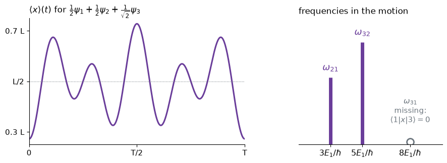

Fig. Left: the average position of the three-state superposition over one period. Right: the frequencies it contains. The two lines are the Bohr frequencies $\omega_{21}$ and $\omega_{32}$ , with heights $2\lvert c_mc_nx_{mn}\rvert$ . The third, $\omega_{31}$ , is missing because $x_{13} = 0$ . Selection rules of this kind decide which lines appear in a spectrum (Chapter 6).

Revivals¶

In a box the energies are $E_n = n^2E_1$ , so every phase $e^{-in^2E_1t/\hbar}$ returns to 1 at the same moment, when $E_1t/\hbar = 2\pi$ . Any state of the box, however complicated, comes back to itself after the revival time

T_{\text{rev}} = \frac{2\pi\hbar}{E_1} = \frac{4mL^2}{\pi\hbar}

(10)

A narrow packet needs many box states (the sine series of Measurement), so between revivals their phases scramble and the packet dissolves. At simple fractions of $T_{\text{rev}}$ the phases partly realign, and the packet comes back in pieces:

# synced: box_revival
import numpy as np
import matplotlib.pyplot as plt
from matplotlib.animation import FuncAnimation
from IPython.display import HTML

TEAL, CARDINAL, GRAY, PURPLE, ORANGE = "#107895", "#C8102E", "#6c757d", "#6a3d9a", "#e07b00"
plt.rcParams.update({"axes.spines.top": False, "axes.spines.right": False})
x = np.linspace(0, 1, 500); dx = x[1] - x[0]               # L = 1; time in units of T_rev = 4 m L^2 / (pi hbar)
ns = np.arange(1, 81)
phis = np.sqrt(2) * np.sin(np.outer(ns, np.pi * x))
g = np.exp(-(x - 0.3)**2 / (4 * 0.05**2)); g = g / np.sqrt(np.sum(g**2) * dx)
c = phis @ g * dx
psi = lambda tau: (c * np.exp(-2j * np.pi * ns**2 * tau)) @ phis
snaps = [(0.0, "t = 0"), (0.01, "t = 0.01 T"), (0.25, "T/4: two copies"), (0.5, "T/2: mirror image"), (1.0, "t = T: back")]
taus = np.linspace(0, 1, 3001)
ret = np.abs(np.exp(-2j * np.pi * np.outer(taus, ns**2)) @ (c**2))**2
fig = plt.figure(figsize=(9.4, 4.1))
gs = fig.add_gridspec(2, len(snaps), height_ratios=[1, 1.15], hspace=0.55, wspace=0.12)
for j, (tau, lab) in enumerate(snaps):
    ax = fig.add_subplot(gs[0, j])
    d = np.abs(psi(tau))**2
    ax.fill_between(x, d, color=CARDINAL, alpha=0.2, lw=0); ax.plot(x, d, color=CARDINAL, lw=1.8)
    ax.plot([0, 0, 1, 1], [8.5, 0, 0, 8.5], color="k", lw=2)
    ax.set_xlim(-0.03, 1.03); ax.set_ylim(0, 8.5); ax.axis("off")
    ax.set_title(lab, fontsize=11.5)
axr = fig.add_subplot(gs[1, :])
axr.plot(taus, ret, color=TEAL, lw=1.3)
for tau, lab in snaps:
    k = int(round(tau * (taus.size - 1)))
    axr.plot([tau], [ret[k]], "o", color=CARDINAL, ms=7, zorder=5)
axr.set_xlim(0, 1); axr.set_ylim(0, 1.08)
axr.set_xticks([0, 0.25, 0.5, 0.75, 1]); axr.set_xticklabels(["0", "T/4", "T/2", "3T/4", "T"], fontsize=11.5)
axr.set_yticks([0, 0.5, 1]); axr.tick_params(labelsize=11)
axr.set_ylabel(r"$|\langle\Psi(0)|\Psi(t)\rangle|^2$", fontsize=12)
axr.set_title("return probability: how much of the starting packet is back", loc="left", fontsize=12.5)
fig.subplots_adjust(left=0.08, right=0.99, top=0.92, bottom=0.11)
plt.show()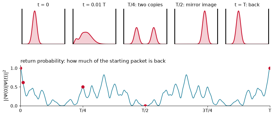

Fig. A narrow packet at rest at $x = 0.3L$ . Top: the density at a few moments. It spreads within a hundredth of the revival time, splits into two copies at $T/4$ , reappears as a mirror image at $T/2$ and is fully restored at $T$ . Bottom: the return probability $\lvert\langle\Psi(0)\vert\Psi(t)\rangle\rvert^2$ , the overlap of the state with where it started, which depends only on the $\lvert c_n\rvert^2$ and the energies.

Chemistry: watching a bond vibrate¶

An ultrashort laser pulse can lift a molecule from its ground vibrational state onto another potential energy curve, where the old ground-state shape is no longer stationary. It becomes a wave packet, a superposition of vibrational states, and it swings back and forth like a classical bond. A second pulse, delayed by a few femtoseconds at a time, takes snapshots of the motion. This is femtochemistry; Ahmed Zewail received the 1999 Nobel Prize in Chemistry for watching bonds vibrate and break this way. In iodine, I₂, the packet swings with a period of about 300 fs.
A real bond is not a harmonic spring. Its potential is closer to a Morse curve, steep when compressed and flattening toward dissociation, and its vibrational levels get closer together as they climb. The clocks of neighboring levels then run at slightly different rates. The packet gradually dephases: it spreads over the whole well and the average bond length stops swinging. The level spacings change by a fixed amount from one level to the next, so the phases realign later and the swing revives:

# synced: morse_revival
import numpy as np
import matplotlib.pyplot as plt
from matplotlib.animation import FuncAnimation
from IPython.display import HTML

TEAL, CARDINAL, GRAY, PURPLE, ORANGE = "#107895", "#C8102E", "#6c757d", "#6a3d9a", "#e07b00"
plt.rcParams.update({"axes.spines.top": False, "axes.spines.right": False})
D = 10.0; a = 1 / np.sqrt(2 * D)                            # hbar = m = 1, harmonic frequency 1 at the bottom
x = np.linspace(-4, 20, 900); dx = x[1] - x[0]
V = D * (1 - np.exp(-a * x))**2
T = -0.5 * (np.eye(x.size, k=1) - 2 * np.eye(x.size) + np.eye(x.size, k=-1)) / dx**2
E, U = np.linalg.eigh(T + np.diag(np.minimum(V, 80))); U = U / np.sqrt(dx)
psi0 = np.exp(-(x + 1.2)**2 / 2) / np.pi**0.25              # ground-state-shaped packet on the compressed side
c = U.T @ psi0 * dx
keep = np.argsort(-c**2)[:30]; cc, UU, EE = c[keep], U[:, keep], E[keep]
X = UU.T @ (x[:, None] * UU) * dx
tl = np.linspace(0, 2 * np.pi * 44, 6000)
A = cc * np.exp(-1j * np.outer(tl, EE))
xm = np.real(np.einsum("ti,ij,tj->t", np.conj(A), X, A))
snaps = [(0.25, "first swings: a compact packet"), (10.3, "about 10 periods: spread out"), (20.25, "about 20 periods: back together")]
fig = plt.figure(figsize=(9.4, 4.4))
gs = fig.add_gridspec(2, 3, height_ratios=[1.1, 1], hspace=0.5, wspace=0.1)
Eav = np.sum(c**2 * E)
for j, (per, lab) in enumerate(snaps):
    ax = fig.add_subplot(gs[0, j])
    d = np.abs(UU @ (cc * np.exp(-1j * EE * per * 2 * np.pi)))**2
    ax.plot(x, V, color=GRAY, lw=1.6)
    ax.fill_between(x, Eav, Eav + 4 * d, color=CARDINAL, alpha=0.2, lw=0); ax.plot(x, Eav + 4 * d, color=CARDINAL, lw=1.8)
    ax.set_xlim(-3, 9); ax.set_ylim(0, 6.2); ax.axis("off")
    ax.set_title(lab, fontsize=11.5)
axm = fig.add_subplot(gs[1, :])
axm.plot(tl / (2 * np.pi), xm, color=TEAL, lw=0.9)
for per, lab in snaps:
    axm.axvline(per, color=CARDINAL, lw=1, ls=":")
axm.set_xlim(0, 44); axm.set_xlabel("time  (vibrational periods)", fontsize=12)
axm.set_ylabel(r"$\langle x\rangle$, bond length", fontsize=11.5); axm.set_yticks([]); axm.tick_params(labelsize=11)
axm.set_title("the average bond length swings, fades as the packet dephases, and comes back", loc="left", fontsize=12.5)
fig.subplots_adjust(left=0.06, right=0.99, top=0.92, bottom=0.12)
plt.show()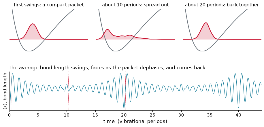

Fig. A ground-state-shaped packet released on the compressed side of a Morse well whose bottom matches a harmonic well. Top: the packet after its first swing, after about 10 periods, and after about 20 periods. Bottom: the average bond length. The swing fades as the packet dephases and returns at about 20 periods; in a harmonic well it would never fade.

The postulates, all together¶

This lecture completes the rules started in Operators 1:

	postulate	in equations
1	the state is a normalized wavefunction	$\langle \psi \vert \psi \rangle = \int \lvert\psi\rvert^2 dx = 1$
2	observables are linear Hermitian operators	$\hat{A} = \hat{A}^\dagger$ , $\ \hat{A}\phi_n = a_n\phi_n$
3	a measurement returns an eigenvalue and leaves its eigenfunction	reading $a_n$ , then $\psi \to \phi_n$
4	outcomes have probabilities; averages are weighted sums	$p_n = \lvert\langle \phi_n \vert \psi \rangle\rvert^2$ , $\ \langle A\rangle = \langle \psi \vert \hat{A} \vert \psi \rangle$
5	the state evolves by the Schrödinger equation	$\Psi(t) = \sum_n c_n e^{-iE_nt/\hbar}\psi_n$

Everything that follows in the course, from the vibrating bond to the hydrogen atom and the chemical bond, applies these five rules to a new $V(x)$ .

Problems¶

Problem 1: Revival times¶

(a) Find the revival time of an electron in boxes 1 nm and 2 nm long. (b) A proton is confined to a well 0.5 Å wide. Treat it as a box and find its revival time. (c) What is the state at half the revival time?

Solution

(a) $T_{\text{rev}} = 4mL^2/\pi\hbar$ grows as $L^2$ : 11 fs for 1 nm, 44 fs for 2 nm.

(b) $T_{\text{rev}} = \dfrac{4\,(1.673\times10^{-27})\,(0.5\times10^{-10})^2}{\pi\,(1.055\times10^{-34})} = 5.0\times10^{-14}\ \text{s} = 50\ \text{fs}$ . The proton is 1836 times heavier, but its box is 20 times narrower, and $1836/400 \approx 4.6$ .

(c) At $T_{\text{rev}}/2$ each phase is $e^{-in^2\pi}= (-1)^{n^2} = (-1)^n$ . A box state is even about the center for odd $n$ and odd for even $n$ , $\psi_n(L - x) = (-1)^{n+1}\psi_n(x)$ , so $\Psi(x, T/2) = -\Psi(L - x, 0)$ : the starting state reflected through the center of the box, as in the figure.

Problem 2: A packet in a uniform field¶

For a particle in a uniform field, $V = mgx$ , use Ehrenfest’s theorem to find $\langle x\rangle(t)$ for a packet that starts at rest at $x_0$ . Does the width of the packet stay constant?

Solution

The force is $-dV/dx = -mg$ everywhere, so its average over the packet is $-mg$ , whatever the packet’s shape:

\frac{d\langle p\rangle}{dt} = -mg, \quad \frac{d\langle x\rangle}{dt} = \frac{\langle p\rangle}{m} \quad\Longrightarrow\quad \langle x\rangle(t) = x_0 - \tfrac{1}{2}gt^2

(12)

The center falls exactly like a classical stone. The width does not stay constant: a uniform force accelerates every part of the packet equally, so it does not stop the spreading of a free packet, and the packet spreads exactly as it would without the field.

Problem 3: Which quantities are conserved?¶

Which of $\hat{p}$ , $\hat{p}^2$ , $\hat{\Pi}$ (parity) and $\hat{H}$ are constants of motion (a) for a free particle, and (b) for a particle on a spring, $V = \frac{1}{2}kx^2$ ?

Solution

(a) Free particle, $\hat{H} = \hat{p}^2/2m$ : all four commute with $\hat{H}$ . Powers of $\hat{p}$ commute with each other, and $\hat{H}$ is unchanged by $x \to -x$ . All four averages are constant.

(b) Spring: $\hat{H}$ is conserved, and so is parity, because $\frac{1}{2}kx^2$ is even. Momentum is not, $[\hat{H},\hat{p}] = i\hbar kx$ , so $d\langle p\rangle/dt = -k\langle x\rangle$ : the spring pushes. Neither is $\hat{p}^2$ : kinetic and potential energy trade back and forth while their sum stays fixed.

Problem 4: Real starting states¶

Show that if $\Psi(x, 0)$ is real, then $\Psi(x, -t) = \Psi^*(x, t)$ , so that $\lvert\Psi(x,t)\rvert^2 = \lvert\Psi(x,-t)\rvert^2$ . What does this say about the motion, and about $\langle p\rangle$ at $t = 0$ ?

Solution

If $\Psi(x,0)$ is real, its coefficients $c_n = \int\psi_n\Psi(x,0)\,dx$ are real (the box states are real). Then

\Psi^*(x,t) = \sum_n c_n\,e^{+iE_nt/\hbar}\,\psi_n(x) = \Psi(x,-t)

(13)

The density at $-t$ equals the density at $t$ : the motion runs the same forward and backward from $t = 0$ , like a ball that is momentarily at rest at the top of its throw. Such a state must have $\langle p\rangle = 0$ at $t = 0$ . Directly: for real $\psi$ , $\langle p\rangle = -i\hbar\int\psi\psi'\,dx = -\frac{i\hbar}{2}\big[\psi^2\big]_{\text{ends}} = 0$ .

Problem 5: Find the revival numerically¶

Adapt the three-line evolver to a box of length $L = 1$ (hard walls, $V = 0$ inside) and start from a narrow Gaussian at $x = 0.3$ . Plot $\lvert\Psi(x,t)\rvert^2$ at $t = 0$ , $T/4$ , $T/2$ and $T$ with $T = 4mL^2/\pi\hbar$ , and compare with the revival figure. How does a finer grid change the result near $T$ , and why?

Problem 6: Two-state beats¶

A particle in a box starts in $\Psi(x,0) = \frac{1}{2}\big(\sqrt{3}\,\psi_1 + \psi_2\big)$ . Find $\lvert\Psi(x,t)\rvert^2$ and $\langle x\rangle(t)$ . What is the period of the motion, and how does the amplitude of $\langle x\rangle$ compare with that of the equal superposition in Particle in a Box?

Problem 7: The swing of iodine¶

The B electronic state of I₂ has vibrational constants $\tilde{\omega}_e = 125.7\ \text{cm}^{-1}$ and $\tilde{\omega}_e x_e = 0.764\ \text{cm}^{-1}$ , so its levels are $E_v/hc = \tilde{\omega}_e(v + \tfrac{1}{2}) - \tilde{\omega}_ex_e(v + \tfrac{1}{2})^2$ . (a) Find the spacing between neighboring levels at $v = 0$ and at $v = 15$ , and the corresponding vibrational periods. (b) Phases of neighboring levels drift apart because the spacing changes by $2\tilde{\omega}_ex_e$ from one pair to the next. Estimate the time after which the packet has dephased, and the time at which the phases realign, $T_{\text{rev}} = 1/(c\,\tilde{\omega}_ex_e)$ .

Problem 8: Parity is forever¶

In a symmetric potential, show that a state that starts even stays even at all times. The equal superposition of $\psi_1$ and $\psi_2$ in a box sloshes from side to side. Why does that not contradict the conservation of parity?