Acknowledgement
The finite-well part of this lecture follows the excellent paper in J. Chem. Educ. 2019, 96, 8, 1663-1670.
A ball bounces back, a wave gets through
Roll a ball toward a hill without enough energy to reach the top and it rolls back, every time. Where the kinetic energy would be negative, so classically the region is forbidden.
A quantum particle is a wave, and the Schrödinger equation does not make a wave vanish where ; it makes it decay (the curvature rule of the Schrödinger equation lecture). If the barrier is thin, the decaying wave reaches the far side with some amplitude left, and there it travels on. The particle can be found beyond a wall it could never climb. That is tunneling.
The animation sends a wavepacket whose energy lies well below the barrier top at a thin barrier, with a classical ball of the same energy for comparison.
Source
# synced: barrier_packet
import numpy as np
import matplotlib.pyplot as plt
from matplotlib.animation import FuncAnimation
from IPython.display import HTML

TEAL, CARDINAL, GRAY, PURPLE, ORANGE = "#107895", "#C8102E", "#6c757d", "#6a3d9a", "#e07b00"
plt.rcParams.update({"axes.spines.top": False, "axes.spines.right": False})
N = 4096                                                    # hbar = m = 1, split-operator steps on a periodic grid
x = np.linspace(-60, 60, N, endpoint=False); dx = x[1] - x[0]
kk = 2 * np.pi * np.fft.fftfreq(N, dx)
k0, V0, a, sig, x0 = 5.0, 20.0, 0.35, 1.5, -14.0             # E = k0^2/2 = 12.5, well below the top V0 = 20
E0 = 0.5 * k0**2
V = np.where((x > 0) & (x < a), V0, 0.0)
psi = np.exp(-(x - x0)**2 / (4 * sig**2) + 1j * k0 * x)
psi = psi / np.sqrt(np.sum(np.abs(psi)**2) * dx)
dt, per, nmove = 0.002, 85, 36                              # each frame advances t by 0.17
half, kin = np.exp(-0.5j * V * dt), np.exp(-0.5j * kk**2 * dt)
dens = np.zeros((nmove, N))
for i in range(nmove):
    dens[i] = np.abs(psi)**2
    for _ in range(per):
        psi = half * np.fft.ifft(kin * np.fft.fft(half * psi))
order = np.concatenate([np.zeros(4, int), np.arange(nmove), np.full(8, nmove - 1)])
thit = (-0.35 - x0) / k0                                    # the classical ball turns at the wall
win = (x > -24) & (x < 24); xs = x[win]
sc = 0.92 * (25.5 - E0) / dens.max()                       # the tallest fringe, at the barrier, just fits
fig, (axc, ax) = plt.subplots(2, 1, figsize=(8, 3.6), sharex=True,
                              gridspec_kw={"height_ratios": [1, 2.7], "hspace": 0.18})
axc.axvspan(0, a, color=GRAY, alpha=0.5, lw=0)
axc.axhline(0.4, color=GRAY, lw=0.8, ls=":")
(ball,) = axc.plot([], [], "o", color=CARDINAL, ms=11)
axc.set_ylim(0, 1); axc.set_yticks([]); axc.spines["left"].set_visible(False); axc.tick_params(bottom=False)
axc.set_title("classical ball with the same energy: it always turns back", loc="left", fontsize=12)
ax.fill_between([0, a], 0, V0, color=GRAY, alpha=0.3, lw=0)
ax.plot([-24, 0, 0, a, a, 24], [0, 0, V0, V0, 0, 0], color="k", lw=2)
ax.axhline(E0, color=GRAY, lw=1, ls="--")
(dline,) = ax.plot([], [], color=TEAL, lw=2)
band = [ax.fill_between(xs, E0, E0, color=TEAL, alpha=0.25, lw=0)]
tlab = ax.text(23.6, 24.6, "", ha="right", va="top", color=TEAL, fontsize=13)
ax.set_xlim(-24, 24); ax.set_ylim(8, 25.5); ax.set_xticks([])
ax.set_yticks([E0, V0]); ax.set_yticklabels(["E", r"$V_0$"], fontsize=13)
ax.set_xlabel("x", fontsize=12)
ax.set_title(r"quantum wave: $|\Psi(x,t)|^2$ drawn on its energy", loc="left", fontsize=12)
fig.subplots_adjust(left=0.06, right=0.98, top=0.92, bottom=0.08)

def update(i):
    d = dens[order[i]]
    t = order[i] * per * dt
    dline.set_data(xs, E0 + sc * d[win])
    band[0].remove(); band[0] = ax.fill_between(xs, E0, E0 + sc * d[win], color=TEAL, alpha=0.25, lw=0)
    ball.set_data([x0 + k0 * t if t < thit else -0.35 - k0 * (t - thit)], [0.4])
    tr = d[x > a].sum() * dx
    tlab.set_text(f"through the barrier: {100 * tr:.0f}%" if tr > 0.005 else "")

ani = FuncAnimation(fig, update, frames=len(order), interval=110, blit=False)
plt.close(fig)
HTML(ani.to_jshtml())Fig. A wavepacket with mean energy meets a thin barrier. Top: a classical ball with the same energy always turns back. Bottom: , drawn on its energy level. Most of the probability reflects, but about a quarter tunnels through and travels on.
Fewer than 1 in 10,000 of the packet’s momentum components carry an energy above , so what gets through is genuinely tunneling, not a leak over the top.
For a short visual overview, here is the Perimeter Institute’s explainer:
Walls of finite height
Everything in this lecture follows from one rule. Rearranged, the time-independent Schrödinger equation reads
Where , the curvature has the opposite sign to : above the axis the curve bends down, below it bends up, so it keeps bending back toward the axis and oscillates. Where , has the same sign as , so the curve bends away from the axis and grows or decays exponentially. The larger , the harder it bends: a shorter wavelength in the first case, a faster decay in the second (see the Schrödinger equation lecture for this rule in pictures).
The walls of the particle in a box are infinitely high, so no particle ever enters them. Real walls, such as the edge of a molecule or the surface of a metal, have a finite height. The simplest model is the finite square well:
A bound state has . Inside the well and the particle is classically allowed; in the walls and it is forbidden.
Inside the well , and the Schrödinger equation is the one we solved for the box:
Its solutions oscillate: .
In the walls :
The sign flip changes everything. The solutions are now the exponentials and , which bend away from the axis. A physical wavefunction must stay finite, so in each wall only the exponential that decays away from the well survives. This decaying piece is not zero: the particle penetrates the wall.
Source
# synced: wall_leak
import numpy as np
import matplotlib.pyplot as plt
from matplotlib.animation import FuncAnimation
from IPython.display import HTML

TEAL, CARDINAL, GRAY, PURPLE, ORANGE = "#107895", "#C8102E", "#6c757d", "#6a3d9a", "#e07b00"
plt.rcParams.update({"axes.spines.top": False, "axes.spines.right": False})
z0 = 2.0                                                    # well strength; x in units of L/2, E in units of V0
lo, hi = 1e-9, np.pi / 2 - 1e-9                             # even ground state: z tan z = sqrt(z0^2 - z^2)
for _ in range(60):
    mid = 0.5 * (lo + hi)
    lo, hi = (mid, hi) if mid * np.tan(mid) < np.sqrt(z0**2 - mid**2) else (lo, mid)
z = 0.5 * (lo + hi); b = np.sqrt(z0**2 - z**2); E = (z / z0)**2    # here beta = b, since L/2 = 1
x = np.linspace(-3.3, 3.3, 900)
psi = np.where(np.abs(x) < 1, np.cos(z * x), np.cos(z) * np.exp(-b * (np.abs(x) - 1)))
sc = 0.42
fig, ax = plt.subplots(figsize=(8, 3.1))
ax.axvspan(-1, 1, color=TEAL, alpha=0.07, lw=0)
for x1, x2 in ((-3.3, -1), (1, 3.3)):
    ax.axvspan(x1, x2, color=CARDINAL, alpha=0.06, lw=0)
ax.plot([-3.3, -1, -1, 1, 1, 3.3], [1, 1, 0, 0, 1, 1], color="k", lw=2.4)
ax.axhline(E, color=GRAY, lw=1.1, ls="--")
ax.text(3.25, E + 0.03, "E", ha="right", va="bottom", color=GRAY, fontsize=13)
ax.fill_between(x, E, E + sc * psi, where=np.abs(x) >= 1, color=CARDINAL, alpha=0.3, lw=0)
ax.plot(x, E + sc * psi, color=TEAL, lw=2.6)
d = 1 / b
ax.annotate("", xy=(1 + d, E - 0.08), xytext=(1, E - 0.08),
            arrowprops=dict(arrowstyle="<->", color=CARDINAL, lw=1.6, shrinkA=0, shrinkB=0))
ax.text(1 + d / 2, E - 0.12, r"$1/\beta$", ha="center", va="top", color=CARDINAL, fontsize=14)
ax.text(1.75, E + 0.14, r"$\psi \propto e^{-\beta x}$", color=CARDINAL, fontsize=13)
ax.text(0, 0.86, r"$V = 0$:  $E > V$, $\psi$ oscillates", ha="center", color=TEAL, fontsize=12.5)
for xc in (-2.15, 2.15):
    ax.text(xc, 1.07, r"$V_0$:  $E < V$, $\psi$ decays", ha="center", color=CARDINAL, fontsize=12.5)
ax.set_xlim(-3.3, 3.3); ax.set_ylim(-0.05, 1.27); ax.set_yticks([])
ax.set_xticks([-1, 0, 1]); ax.set_xticklabels([r"$-L/2$", "0", r"$L/2$"], fontsize=13)
ax.spines["left"].set_visible(False)
fig.tight_layout()
plt.show()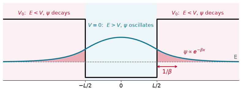
Fig. The ground state of a finite well, drawn on its energy level. Inside the well oscillates; in the walls it decays as . The shaded tails are probability in the classically forbidden region, and marks the penetration depth.
A number worth remembering: for an electron, .
Reading a wavefunction from its potential
The same rules give the shape of in any potential made of steps. Where is large the curvature is strong and the wavelength short; where is large the decay is fast; and at every step and its slope join smoothly.
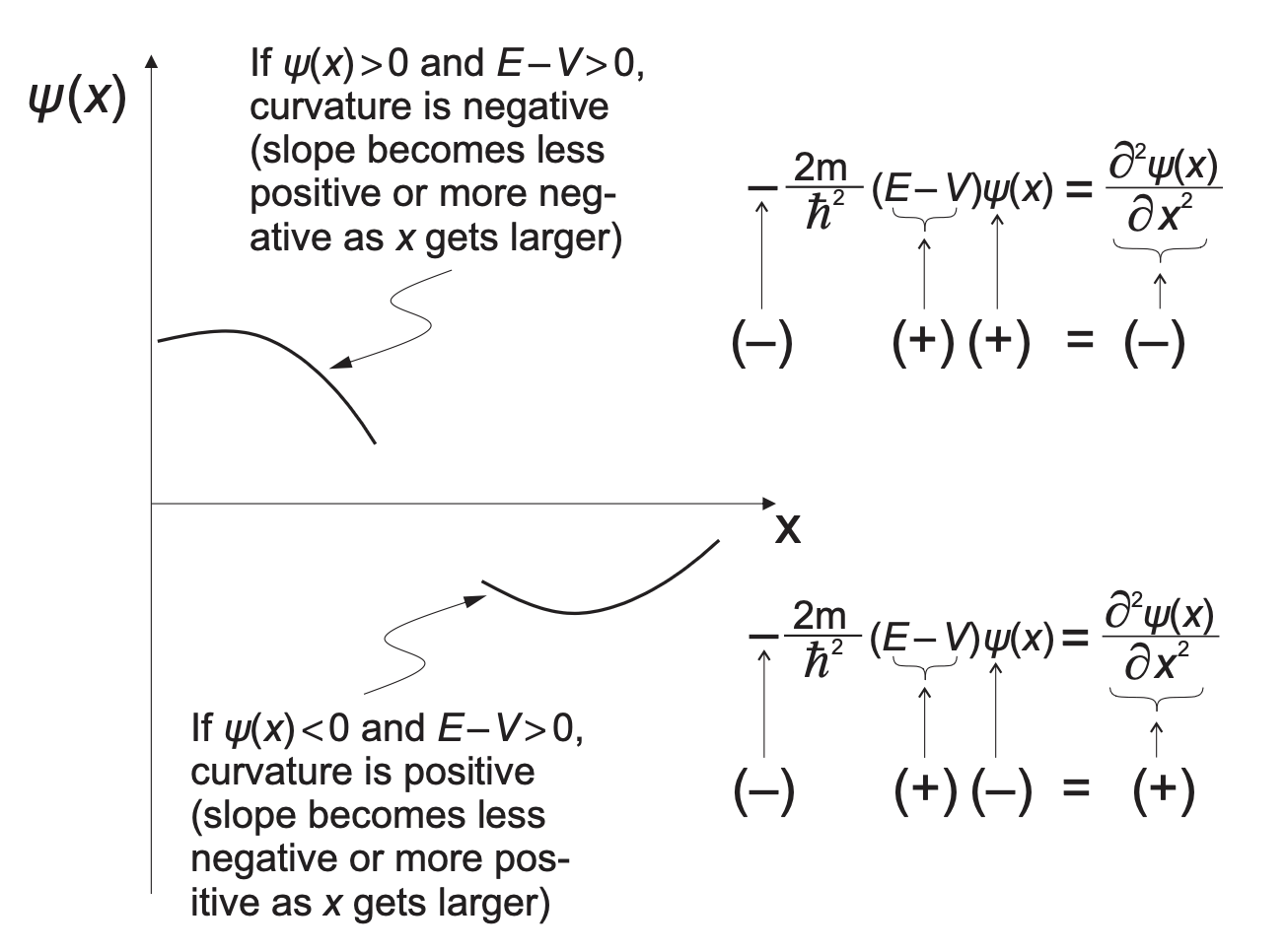
Figure 1:A stepped potential (top) and the wavefunction it produces (bottom). Large gives a short wavelength and a small amplitude, small gives a slow decay, and the slopes match at every step.
Joining the pieces
With far from the well, the wavefunction in the three regions is
Why both and must be continuous. A jump in would leave the probability density undefined at the joint. A kink, a jump in , would make infinite there, and is what the kinetic energy operator acts on. A finite energy cannot produce an infinite curvature unless the potential is infinite. The infinite box is that exception: its walls allow a kink, which is why we required only there.
This gives four conditions, two at each wall:
At most energies the values can be matched but the slopes cannot: the joined function has a kink and does not solve the Schrödinger equation. Only at special energies do both match.
Source
# synced: fsw_match
import numpy as np
import matplotlib.pyplot as plt
from matplotlib.animation import FuncAnimation
from IPython.display import HTML

TEAL, CARDINAL, GRAY, PURPLE, ORANGE = "#107895", "#C8102E", "#6c757d", "#6a3d9a", "#e07b00"
plt.rcParams.update({"axes.spines.top": False, "axes.spines.right": False})
z0 = 2.0                                                    # the same well as wall_leak
lo, hi = 1e-9, np.pi / 2 - 1e-9
for _ in range(60):
    mid = 0.5 * (lo + hi)
    lo, hi = (mid, hi) if mid * np.tan(mid) < np.sqrt(z0**2 - mid**2) else (lo, mid)
zr = 0.5 * (lo + hi)
x = np.linspace(-2.6, 2.6, 900)
fig, axes = plt.subplots(2, 1, figsize=(4.8, 4.4), sharex=True, gridspec_kw={"hspace": 0.45})
for ax, z, col, head in ((axes[0], 0.45 * zr, CARDINAL, "trial E: the slopes disagree, a kink"),
                         (axes[1], zr, TEAL, r"allowed E: $\psi$ and $\psi'$ both match")):
    b = np.sqrt(z0**2 - z**2); E = (z / z0)**2
    psi = np.where(np.abs(x) < 1, np.cos(z * x), np.cos(z) * np.exp(-b * (np.abs(x) - 1)))
    ax.plot([-2.6, -1, -1, 1, 1, 2.6], [1, 1, 0, 0, 1, 1], color="k", lw=2)
    ax.axhline(E, color=GRAY, lw=0.9, ls="--")
    ax.plot(x, E + 0.45 * psi, color=col, lw=2.6)
    ax.plot([-1, 1], [E + 0.45 * np.cos(z)] * 2, "o", mfc="none", mec=col, mew=2, ms=17)
    ax.set_title(head, loc="left", fontsize=12.5, color=col)
    ax.set_xlim(-2.6, 2.6); ax.set_ylim(-0.04, 1.08); ax.set_yticks([])
    ax.spines["left"].set_visible(False)
axes[0].tick_params(bottom=False)
axes[1].set_xticks([-1, 0, 1]); axes[1].set_xticklabels([r"$-L/2$", "0", r"$L/2$"], fontsize=12)
fig.subplots_adjust(left=0.03, right=0.98, top=0.92, bottom=0.1)
plt.show()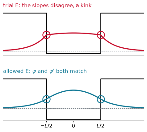
Fig. A cosine inside the well joined to decaying exponentials in the walls, with the values matched. Top: at a trial energy the slopes disagree, leaving a kink at each wall. Bottom: at the allowed energy the value and the slope both match.
Even and odd states
The well is symmetric about , so every state is either even, , or odd, . Inside the well the even states are cosines and the odd states are sines. Each family then needs only the matching at ; the wall at follows by symmetry.
Even states. Inside the well , and in the right wall . Differentiate each piece to get its slope:
Now require that the values agree and that the slopes agree at :
Dividing the slope equation by the value equation removes the unknown amplitudes and , and leaves a condition on the energy alone:
Odd states. Match in the same way, and , so
Counting up the ladder, the even states are and the odd states are : cosines and sines take turns, as they do in a box centered on the origin.
Both and depend on , so these are transcendental equations: no algebra isolates . Their structure shows up in units of the half width. Define
Because does not depend on , the two unknowns lie on a circle, .
Finding the energies graphically
Plot the even branches and the odd branches against , and draw the quarter circle of radius . Every crossing is a bound state.
The branches start on the axis at , alternating even and odd, and each one rises without limit. The circle crosses every branch that starts below , so the number of bound states is
One more state appears each time grows past a multiple of . The first even branch starts at the origin, so every finite well, however shallow or narrow, holds at least one bound state. This is a one-dimensional fact: in three dimensions a weak enough well binds nothing.
Change the depth and the width of the well for an electron below. The left panel is the graphical solution; the right panel shows the levels in the well, with the levels of an infinite box of the same width dashed.
Fig. Left: the graphical solution, with the even branches in teal and the odd branches in purple crossed by the circle of radius . Right: the resulting levels of an electron in the well, with the levels of an infinite box of the same width dashed in gray.
Here are some questions to think about:
Q1: How does changing the width affect the number and the energies of the states?
Q2: How does changing the depth affect them?
Q3: Is the ground state even or odd? Could it ever be the other kind?
Q4: What is the smallest number of bound states a well can have?
Q5: Do the levels follow the infinite-box pattern ? Where does the pattern fail first?
Wavefunctions and the probability of leaking out
With the energies known, the matching conditions give the amplitudes, and normalization fixes the last constant. The figure shows the four bound states of an electron in a well 10 Å wide and 5 eV deep, for which .
Source
# synced: fsw_ladder
import numpy as np
import matplotlib.pyplot as plt
from matplotlib.animation import FuncAnimation
from IPython.display import HTML

TEAL, CARDINAL, GRAY, PURPLE, ORANGE = "#107895", "#C8102E", "#6c757d", "#6a3d9a", "#e07b00"
plt.rcParams.update({"axes.spines.top": False, "axes.spines.right": False})
V0, L = 5.0, 10.0                                           # electron in a 5 eV, 10 Angstrom well (the page's example)
z0 = 0.5 * L * 0.5123 * np.sqrt(V0)                         # 0.5123 = sqrt(2 m_e (1 eV)) / hbar, in 1/Angstrom
n = int(2 * z0 / np.pi) + 1
zs = np.zeros(n)
for m in range(n):
    lo, hi = m * np.pi / 2 + 1e-9, min((m + 1) * np.pi / 2, z0) - 1e-9
    for _ in range(60):
        mid = 0.5 * (lo + hi)
        f = (mid * np.tan(mid) if m % 2 == 0 else -mid / np.tan(mid)) - np.sqrt(z0**2 - mid**2)
        lo, hi = (mid, hi) if f < 0 else (lo, mid)
    zs[m] = 0.5 * (lo + hi)
E = V0 * (zs / z0)**2
Einf = 0.3760 * np.arange(1, n + 1)**2                      # n^2 h^2 / 8 m L^2 for L = 10 Angstrom, in eV
x = np.linspace(-12, 12, 1600); dx = x[1] - x[0]
out = np.abs(x) > L / 2
fig, (ax1, ax2, ax3) = plt.subplots(1, 3, figsize=(8, 3.6), sharey=True,
                                    gridspec_kw={"width_ratios": [1, 1, 0.5], "wspace": 0.08})
for ax in (ax1, ax2):
    ax.plot([-12, -5, -5, 5, 5, 12], [V0, V0, 0, 0, V0, V0], color="k", lw=2.2)
    ax.set_xlim(-12, 12); ax.set_xticks([-5, 5]); ax.set_xticklabels([r"$-L/2$", r"$L/2$"], fontsize=12)
for m in range(n):
    k, b = 2 * zs[m] / L, 2 * np.sqrt(z0**2 - zs[m]**2) / L
    if m % 2 == 0:
        psi = np.where(out, np.cos(k * L / 2) * np.exp(-b * (np.abs(x) - L / 2)), np.cos(k * x))
    else:
        psi = np.where(out, np.sign(x) * np.sin(k * L / 2) * np.exp(-b * (np.abs(x) - L / 2)), np.sin(k * x))
    p = psi**2 / (np.sum(psi**2) * dx)
    col = TEAL if m % 2 == 0 else PURPLE
    for ax in (ax1, ax2):
        ax.hlines(E[m], -12, 12, color=GRAY, lw=0.8, ls="--")
    ax1.plot(x, E[m] + 0.36 * psi / np.abs(psi).max(), color=col, lw=2.2)
    pn = 0.6 * p / p.max()
    ax2.fill_between(x, E[m], E[m] + pn, where=out, color=CARDINAL, alpha=0.5, lw=0)
    ax2.plot(x, E[m] + pn, color=CARDINAL, lw=1.8)
    ax2.text(11.8, E[m] + 0.08, f"{100 * np.sum(p[out]) * dx:.1f}%", ha="right", va="bottom",
             fontsize=11.5, color=CARDINAL)
    ax3.plot([0.06, 0.42], [E[m]] * 2, color=col, lw=3)
    ax3.plot([0.58, 0.94], [Einf[m]] * 2, color=GRAY, lw=3)
    ax3.plot([0.42, 0.58], [E[m], Einf[m]], color=GRAY, lw=0.9, ls=":")
ax3.axhline(V0, color="k", lw=1.6)
ax3.set_xlim(0, 1); ax3.set_xticks([0.24, 0.76]); ax3.set_xticklabels(["finite", "infinite"], fontsize=11.5)
ax3.tick_params(bottom=False)
ax1.set_ylim(-0.15, 6.5); ax1.set_yticks(range(7)); ax1.set_ylabel("energy (eV)", fontsize=12)
ax1.set_title(r"$\psi_n$ on its level", loc="left", fontsize=12)
ax2.set_title(r"$|\psi_n|^2$, shaded: outside", loc="left", fontsize=12)
ax3.set_title("levels", loc="left", fontsize=12)
for ax in (ax2, ax3):
    ax.tick_params(left=False)
fig.subplots_adjust(left=0.08, right=0.99, top=0.91, bottom=0.1)
plt.show()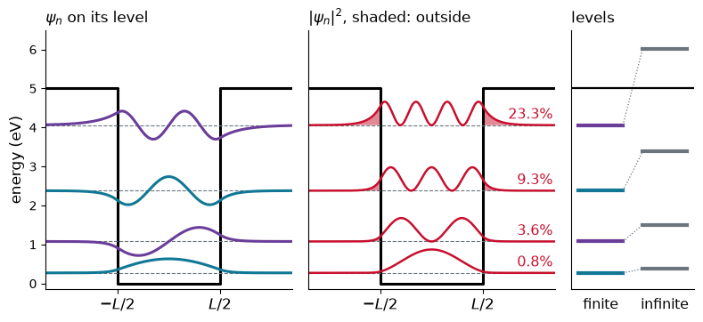
Fig. The four bound states of an electron in a finite well 5 eV deep and 10 Å wide. Left: drawn on its level, even states in teal and odd states in purple. Middle: , with the probability in the walls shaded and quoted. Right: the finite-well levels against those of an infinite box of the same width.
The tunneling probability is the shaded area, the chance of finding the particle outside the well. For a normalized ,
grows from under 1% for the ground state to 23% for the top state. The closer a level is to the rim, the smaller its and the deeper it leaks: the penetration depths here are 0.90, 0.99, 1.21 and 2.01 Å.
Finite versus infinite. Every finite-well level lies below its infinite-box partner: 0.27 eV against 0.38 eV for , and 4.06 eV against 6.02 eV for . Leaking into the walls gives the wave more room, so its wavelength is longer, its is smaller, and its energy is lower. The effect is largest near the top, where the leak is largest. Low in the well the wave barely penetrates, and the levels nearly match the infinite box.
Tunneling through a barrier
Turn the finite well upside down. A barrier of height and width ,
meets a particle that comes in from the left with . The particle is free on both sides, so nothing quantizes its energy. The question now is what fraction of the incoming wave gets through.
In the three regions,
with the same and as before. Inside the barrier both exponentials stay, since neither can blow up over a finite width. On the right there is only an outgoing wave, because nothing comes in from the right.
What the transmission coefficient means. Send many particles at the barrier, all prepared the same way. Each one is detected either on the left (reflected) or on the right (transmitted), never half and half. The transmission coefficient is the fraction found on the right; for a single particle it is the probability of getting through. The reflection coefficient is the fraction found on the left, and .
How to get from the wave. A traveling wave carries a probability flux, the probability crossing a point per second: its density times its speed . is the ratio of the transmitted flux to the incident flux. The incident wave has amplitude 1, and the speed is the same on both sides of the barrier, so the speeds cancel:
Source
# synced: barrier_setup
import numpy as np
import matplotlib.pyplot as plt
from matplotlib.animation import FuncAnimation
from IPython.display import HTML

TEAL, CARDINAL, GRAY, PURPLE, ORANGE = "#107895", "#C8102E", "#6c757d", "#6a3d9a", "#e07b00"
plt.rcParams.update({"axes.spines.top": False, "axes.spines.right": False})
E, V0, a = 0.5, 1.0, 1.0                                    # hbar = m = 1: k = beta = 1, so T = sech^2(1) = 0.42
k, q = np.sqrt(2 * E), np.sqrt(2 * (V0 - E))
M = np.array([[1, -1, -1, 0], [-1j * k, -q, q, 0],
              [0, np.exp(q * a), np.exp(-q * a), -np.exp(1j * k * a)],
              [0, q * np.exp(q * a), -q * np.exp(-q * a), -1j * k * np.exp(1j * k * a)]])
r, C, D, t = np.linalg.solve(M, np.array([-1, -1j * k, 0, 0]))
R, T = abs(r)**2, abs(t)**2
fig, ax = plt.subplots(figsize=(8, 3.3))
ax.fill_between([0, a], 0, 1, color=GRAY, alpha=0.3, lw=0)
ax.plot([-9.5, 0, 0, a, a, 10.5], [0, 0, 1, 1, 0, 0], color="k", lw=2)
ax.text(a / 2, 1.04, r"$V_0$", ha="center", va="bottom", fontsize=13)
xl, xr = np.linspace(-9.3, -0.4, 400), np.linspace(a + 0.4, 10.3, 400)
w = 0.1                                                     # drawn amplitude of a unit wave
ax.plot(xl, 0.8 + w * np.cos(k * xl), color=TEAL, lw=2.4)
ax.plot(xl, 0.28 + w * abs(r) * np.cos(-k * xl + np.angle(r)), color=ORANGE, lw=2.4)
ax.plot(xr, 0.55 + w * abs(t) * np.cos(k * xr + np.angle(t)), color=TEAL, lw=2.4)
for (x1, x2), y, f, c in (((-7.5, -2.5), 0.62, 1.0, TEAL), ((-2.5, -7.5), 0.1, R, ORANGE), ((3.0, 8.0), 0.37, T, TEAL)):
    ax.annotate("", xy=(x2, y), xytext=(x1, y), arrowprops=dict(
        arrowstyle=f"simple,head_length=0.8,head_width={0.4 + 1.1 * f:.2f},tail_width={0.6 * f:.2f}",
        color=c, alpha=0.75, mutation_scale=22))
ax.text(-9.3, 0.96, r"incident $e^{ikx}$: flux 1", fontsize=12.5, color=TEAL, va="bottom")
ax.text(-9.3, 0.42, rf"reflected $r\,e^{{-ikx}}$: $R = |r|^2 = {R:.2f}$", fontsize=12.5, color=ORANGE, va="bottom")
ax.text(10.3, 0.69, rf"transmitted $t\,e^{{ikx}}$: $T = |t|^2 = {T:.2f}$", fontsize=12.5, color=TEAL,
        va="bottom", ha="right")
ax.set_xlim(-9.5, 10.5); ax.set_ylim(-0.05, 1.2); ax.axis("off")
fig.subplots_adjust(left=0.01, right=0.99, top=0.98, bottom=0.02)
plt.show()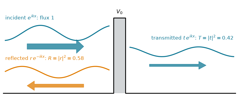
Fig. The three pieces of the wave at a barrier with and width . The incident wave has amplitude 1. The reflected wave carries back the fraction of the incident flux, and the transmitted wave carries on with ; the widths of the arrows show the flux.
The four matching conditions, and continuous at and at , fix , , and . The algebra is long, but the result is compact:
For a thick barrier , which gives the second form. Its prefactor is of order one; the exponential does the work. The amplitude falls by across the barrier, and the probability by its square.
Source
# synced: barrier_width
import numpy as np
import matplotlib.pyplot as plt
from matplotlib.animation import FuncAnimation
from IPython.display import HTML

TEAL, CARDINAL, GRAY, PURPLE, ORANGE = "#107895", "#C8102E", "#6c757d", "#6a3d9a", "#e07b00"
plt.rcParams.update({"axes.spines.top": False, "axes.spines.right": False})
E, V0 = 0.5, 1.0                                            # hbar = m = 1: k = beta = 1, so the exact T is sech^2(a)
k, q = np.sqrt(2 * E), np.sqrt(2 * (V0 - E))
x = np.linspace(-12.5, 15.5, 1400)
nf = 44
aa = np.concatenate([np.linspace(0.15, 3.0, nf - 10), np.full(10, 3.0)])
ph = 2 * np.pi * np.arange(nf) / 11                         # e^{-i omega t}: one turn every 11 frames
ag = np.linspace(0, 3.2, 200)
fig, (ax, axt) = plt.subplots(1, 2, figsize=(8, 3.0), gridspec_kw={"width_ratios": [2.4, 1], "wspace": 0.22})
(pot,) = ax.plot([], [], color="k", lw=2)
blk = [ax.fill_between([0, 1], 0, 1, color=GRAY, alpha=0.25, lw=0)]
ax.axhline(E, color=GRAY, lw=1, ls="--")
(wave,) = ax.plot([], [], color=TEAL, lw=2.2)
(envp,) = ax.plot([], [], color=TEAL, lw=1.1, ls=":")
(envm,) = ax.plot([], [], color=TEAL, lw=1.1, ls=":")
ax.text(-6.5, 1.06, "incident + reflected", ha="center", color=GRAY, fontsize=12)
ax.text(9.5, 1.06, r"transmitted, amplitude $|t|$", ha="center", color=TEAL, fontsize=12)
ax.set_xlim(-12.5, 15.5); ax.set_ylim(-0.02, 1.2); ax.set_xticks([])
ax.set_yticks([E, V0]); ax.set_yticklabels(["E", r"$V_0$"], fontsize=13)
ax.set_xlabel("x", fontsize=12)
axt.semilogy(ag, 1 / np.cosh(ag)**2, color=GRAY, lw=2.2)
axt.semilogy(ag, 4 * np.exp(-2 * ag), color=GRAY, lw=1, ls="--")
axt.text(1.45, 0.55, r"$\approx 4\,e^{-2\beta a}$", fontsize=12, color=GRAY)
(dot,) = axt.plot([], [], "o", color=CARDINAL, ms=9, zorder=5)
axt.set_xlim(0, 3.2); axt.set_ylim(5e-3, 1.6)
axt.set_xlabel(r"width $a$, units of $1/\beta$", fontsize=11.5)
axt.set_title(r"$T$, log scale", loc="left", fontsize=12)
fig.subplots_adjust(left=0.05, right=0.98, top=0.88, bottom=0.17)

def update(i):
    a = aa[i]
    M = np.array([[1, -1, -1, 0], [-1j * k, -q, q, 0],                     # psi and psi' continuous at 0 and a
                  [0, np.exp(q * a), np.exp(-q * a), -np.exp(1j * k * a)],
                  [0, q * np.exp(q * a), -q * np.exp(-q * a), -1j * k * np.exp(1j * k * a)]])
    r, C, D, t = np.linalg.solve(M, np.array([-1, -1j * k, 0, 0]))
    psi = np.where(x < 0, np.exp(1j * k * x) + r * np.exp(-1j * k * x),
                   np.where(x < a, C * np.exp(q * x) + D * np.exp(-q * x), t * np.exp(1j * k * x)))
    wave.set_data(x, E + 0.2 * np.real(psi * np.exp(-1j * ph[i])))
    xr = x[x >= a]
    envp.set_data(xr, E + 0.2 * abs(t) + 0 * xr); envm.set_data(xr, E - 0.2 * abs(t) + 0 * xr)
    pot.set_data([-12.5, 0, 0, a, a, 15.5], [0, 0, V0, V0, 0, 0])
    blk[0].remove(); blk[0] = ax.fill_between([0, a], 0, V0, color=GRAY, alpha=0.25, lw=0)
    dot.set_data([a], [abs(t)**2])
    ax.set_title(rf"$a = {a:.2f}/\beta$:  $T = |t|^2 = {abs(t)**2:.3f}$", loc="left", fontsize=13)

ani = FuncAnimation(fig, update, frames=nf, interval=120, blit=False)
plt.close(fig)
HTML(ani.to_jshtml())Fig. A wave with energy meets a barrier that slowly widens. Left: the real part of the wave as it oscillates in time, incident plus reflected on the left, decaying inside the barrier, and transmitted with amplitude on the right. Right: on a log scale, where the exponential becomes a straight line.
Some books, and section 7 of the Python calculator, write for . The calculator also follows above the barrier top, where a classical particle always passes but a quantum one can still reflect.
Width and mass sit in the exponent
Because , both the width and the square root of the mass sit in the exponent of . Each extra ångström of barrier multiplies by the same factor, and a heavier particle has a larger . A proton is 1836 times heavier than an electron, so its is times larger.
Compare an electron, a proton (H) and a deuteron (D) facing the same barrier:
Fig. against the barrier width for an electron, a proton and a deuteron facing the same barrier, on a log scale. The dots mark the chosen width.
Electrons tunnel through barriers nanometers wide. This is how electrons hop between metal centers in proteins and through thin insulating films. Protons and hydrogen atoms tunnel only through barriers a fraction of an ångström wide, which happens to be about the distance a hydrogen moves when it transfers between two atoms in a reaction.
Tunneling at work
The scanning tunneling microscope
In a scanning tunneling microscope (STM) a sharp metal tip hovers a few ångströms above a conducting surface. The vacuum gap is a barrier whose height is set by the work function , the energy needed to pull an electron out of the metal (4 to 5 eV). A small voltage drives electrons across the gap by tunneling, and the current falls exponentially with the gap :
Scanning the tip across the surface while recording the current maps the surface atom by atom. Gerd Binnig and Heinrich Rohrer built the first STM at IBM Zurich in 1981 and shared the 1986 Nobel Prize in Physics for it.
Source
# synced: stm_scan
import numpy as np
import matplotlib.pyplot as plt
from matplotlib.animation import FuncAnimation
from IPython.display import HTML

TEAL, CARDINAL, GRAY, PURPLE, ORANGE = "#107895", "#C8102E", "#6c757d", "#6a3d9a", "#e07b00"
plt.rcParams.update({"axes.spines.top": False, "axes.spines.right": False})
beta, h = 1.09, 3.6                                         # 1/Angstrom for a 4.5 eV work function; apex height
cx = np.append(1.5 + 3.0 * np.arange(6), 12.0)              # six surface atoms and one adatom in a hollow
cy = np.append(np.zeros(6), 1.2)
R = np.append(np.full(6, 1.0), 0.8)                         # the adatom's top sits 1 Angstrom above the others
xs = np.linspace(-0.2, 18.2, 1500)
gap = (np.sqrt((xs[:, None] - cx)**2 + (h - cy)**2) - R).min(axis=1)
cur = np.exp(-2 * beta * (gap - (h - 1.0)))                 # current relative to the value over a surface atom
nf = 46
xt = np.concatenate([np.linspace(-0.2, 18.2, nf - 6), np.full(6, 18.2)])
fig, (ax, axi) = plt.subplots(2, 1, figsize=(8, 3.8), sharex=True,
                              gridspec_kw={"height_ratios": [2.0, 1], "hspace": 0.14})
for x0, y0, r0, c in zip(cx, cy, R, [GRAY] * 6 + [ORANGE]):
    ax.add_patch(plt.Circle((x0, y0), r0, facecolor=c, alpha=0.45 if c == GRAY else 0.85, edgecolor=c, lw=1.5))
tip = plt.Polygon([[0, h], [-1.6, h + 3.2], [1.6, h + 3.2]], closed=True, facecolor=GRAY, edgecolor="k", lw=1.2)
ax.add_patch(tip)
(spark,) = ax.plot([], [], color=TEAL, solid_capstyle="round")
ax.set_aspect("equal"); ax.set_xlim(-0.2, 18.2); ax.set_ylim(-0.6, 5.4); ax.axis("off")
ax.set_title("the tip scans at constant height; electrons tunnel across the gap", loc="left", fontsize=13)
axi.plot(xs, cur, color=TEAL, lw=1, alpha=0.15)
(trace,) = axi.plot([], [], color=TEAL, lw=2.4)
(now,) = axi.plot([], [], "o", color=TEAL, ms=7)
axi.set_ylim(0, 10); axi.set_yticks([0, 4, 8]); axi.set_xticks([]); axi.tick_params(labelsize=12)
axi.set_ylabel("current", fontsize=13)
fig.subplots_adjust(left=0.07, right=0.99, top=0.93, bottom=0.04)

def update(i):
    x0 = xt[i]
    tip.set_xy([[x0, h], [x0 - 1.6, h + 3.2], [x0 + 1.6, h + 3.2]])
    j = np.argmin(np.sqrt((x0 - cx)**2 + (h - cy)**2) - R)   # nearest atom: the electrons tunnel to it
    u = np.array([x0 - cx[j], h - cy[j]]); u = u / np.linalg.norm(u)
    I = np.interp(x0, xs, cur)
    spark.set_data([x0, cx[j] + R[j] * u[0]], [h, cy[j] + R[j] * u[1]])
    spark.set_linewidth(1.2 + 1.8 * I**0.6); spark.set_alpha(min(1.0, 0.35 + 0.12 * I))
    ok = xs <= x0
    trace.set_data(xs[ok], cur[ok]); now.set_data([x0], [I])

ani = FuncAnimation(fig, update, frames=nf, interval=110, blit=False)
plt.close(fig)
HTML(ani.to_jshtml())Fig. A tip scans at constant height over a row of surface atoms (gray) and one adatom (orange) whose top sits 1 Å higher. The tunneling current, drawn below, follows the gap exponentially: the adatom gives about nine times the current of a surface atom.
Ammonia turns inside out
Ammonia is a pyramid: the nitrogen sits above the plane of the three hydrogens like the handle of an umbrella. Pushing the nitrogen through that plane gives the mirror-image pyramid, with the same energy. Along this umbrella coordinate the potential is a double well, two equal minima separated by a barrier of about 0.25 eV at the planar geometry.
If the barrier were infinite, each well would hold its own ground state, and the two would have exactly the same energy. Tunneling through the barrier couples them. The true stationary states are the even and odd combinations, which spread over both wells, and their energies split by a small amount . This is the tunneling doublet you can find with the numerical Schrödinger solver.
A molecule prepared in one pyramid, the left well, is the superposition . Exactly as for the sloshing particle in a box of the previous lecture, the cross term makes the probability oscillate, here between the two wells: the molecule tunnels to the other pyramid and back with period .
Source
# synced: ammonia_flip
import numpy as np
import matplotlib.pyplot as plt
from matplotlib.animation import FuncAnimation
from IPython.display import HTML

TEAL, CARDINAL, GRAY, PURPLE, ORANGE = "#107895", "#C8102E", "#6c757d", "#6a3d9a", "#e07b00"
plt.rcParams.update({"axes.spines.top": False, "axes.spines.right": False})
Vb, N = 14.0, 700                                           # V = Vb (x^2 - 1)^2 with H = -d^2/dx^2 + V
x = np.linspace(-2.2, 2.2, N); h = x[1] - x[0]
V = Vb * (x**2 - 1)**2
H = np.diag(2 / h**2 + V) - np.diag(np.ones(N - 1) / h**2, 1) - np.diag(np.ones(N - 1) / h**2, -1)
En, vec = np.linalg.eigh(H)
s, an = vec[:, 0] / np.sqrt(h), vec[:, 1] / np.sqrt(h)
s = s * np.sign(s[N // 2]); an = an * np.sign(an[N // 4])  # an > 0 on the left, so s + an starts on the left
D, Em = En[1] - En[0], 0.5 * (En[0] + En[1])
nf = 44
ph = 2 * np.pi * np.arange(nf) / nf                         # Delta t over one full period h/Delta, a seamless loop
rho0 = 0.5 * (s + an)**2
sc = 0.36 * Vb / rho0.max()
fig = plt.figure(figsize=(8, 3.6))
gs = fig.add_gridspec(1, 2, width_ratios=[2.2, 1], wspace=0.22)
ax, axp = fig.add_subplot(gs[0]), fig.add_subplot(gs[1])
ax.plot(x, V, color="k", lw=2)
ax.axhline(En[0], color=TEAL, lw=1.2); ax.axhline(En[1], color=PURPLE, lw=1.2)
ax.annotate(r"split by $\Delta$", xy=(0, En[0] - 0.1), xytext=(0, 3.2), ha="center", fontsize=12, color=GRAY,
            arrowprops=dict(arrowstyle="->", color=GRAY, lw=1.2))
(dline,) = ax.plot([], [], color=TEAL, lw=2)
band = [ax.fill_between(x, Em, Em, color=TEAL, alpha=0.25, lw=0)]
ax.set_xlim(-2.2, 2.2); ax.set_ylim(0, 1.75 * Vb); ax.set_xticks([]); ax.set_yticks([])
ax.set_xlabel("umbrella coordinate", fontsize=12); ax.set_ylabel("energy", fontsize=12)
ax.set_title("start on the left: it tunnels across and back", loc="left", fontsize=12)
axp.axhline(0.5, color=GRAY, lw=0.7, ls=":")
(trace,) = axp.plot([], [], color=TEAL, lw=2.4)
(now,) = axp.plot([], [], "o", color=TEAL, ms=7)
axp.set_xlim(0, 1); axp.set_ylim(-0.04, 1.06)
axp.set_xticks([0, 0.5, 1]); axp.set_xticklabels(["0", r"$h/2\Delta$", r"$h/\Delta$"], fontsize=12)
axp.set_yticks([0, 1]); axp.set_yticklabels(["0", "1"], fontsize=12); axp.set_xlabel("time", fontsize=12)
axp.set_title("probability on the right", loc="left", fontsize=12)
fig.subplots_adjust(left=0.05, right=0.98, top=0.9, bottom=0.15)
p = ax.get_position()
mols = []                                                   # NH3 seen side on: N above (left well) or below (right)
for xc, sg in ((-1.0, 1), (1.0, -1)):
    u = (xc + 2.2) / 4.4
    axm = fig.add_axes([p.x0 + p.width * u - 0.07, p.y0 + p.height * 0.68, 0.14, 0.24])
    axm.set_xlim(-1, 1); axm.set_ylim(-1, 1); axm.set_aspect("equal"); axm.axis("off")
    hx, hy = np.array([-0.62, 0.62, 0.16]), sg * np.array([-0.18, -0.18, -0.42])
    bonds = [axm.plot([0, hx[j]], [sg * 0.5, hy[j]], color=GRAY, lw=2.2)[0] for j in range(3)]
    hs = axm.scatter(hx, hy, s=170, facecolor="white", edgecolor=GRAY, lw=1.6, zorder=3)
    nn = axm.scatter([0], [sg * 0.5], s=420, facecolor=TEAL, edgecolor="k", lw=1, zorder=4)
    mols.append(bonds + [hs, nn])
xg = np.linspace(0, 1, 300)
pr = np.sum((s * an)[x > 0]) * h                            # P_right(t) = 1/2 + pr cos(Delta t), pr close to -1/2

def update(i):
    c = np.cos(ph[i])
    rho = 0.5 * (s**2 + an**2) + s * an * c                 # |Psi|^2: a fixed part and a cross term at frequency Delta
    dline.set_data(x, Em + sc * rho)
    band[0].remove(); band[0] = ax.fill_between(x, Em, Em + sc * rho, color=TEAL, alpha=0.25, lw=0)
    Pr = 0.5 + pr * c
    for art in mols[0]:
        art.set_alpha(0.12 + 0.88 * (1 - Pr))
    for art in mols[1]:
        art.set_alpha(0.12 + 0.88 * Pr)
    tt = i / nf
    ok = xg <= tt
    trace.set_data(xg[ok], 0.5 + pr * np.cos(2 * np.pi * xg[ok])); now.set_data([tt], [Pr])

ani = FuncAnimation(fig, update, frames=nf, interval=100, blit=False)
plt.close(fig)
HTML(ani.to_jshtml())Fig. A molecule starts in the left well of a double well. Its density , drawn on the energy of the doublet, tunnels to the right well and back with period , set by the splitting of the even and odd levels. Right: the probability of finding the molecule in the right well.
For NH₃ the splitting is , a frequency of about 24 GHz: the umbrella flips across and back every 42 ps. Microwaves of this frequency, with a wavelength of about 1.26 cm, drive transitions between the two levels of the doublet. Charles Townes used them in 1954 to build the first maser, the microwave ancestor of the laser. In ND₃ the heavier deuterons tunnel 15 times more slowly ().
More tunneling
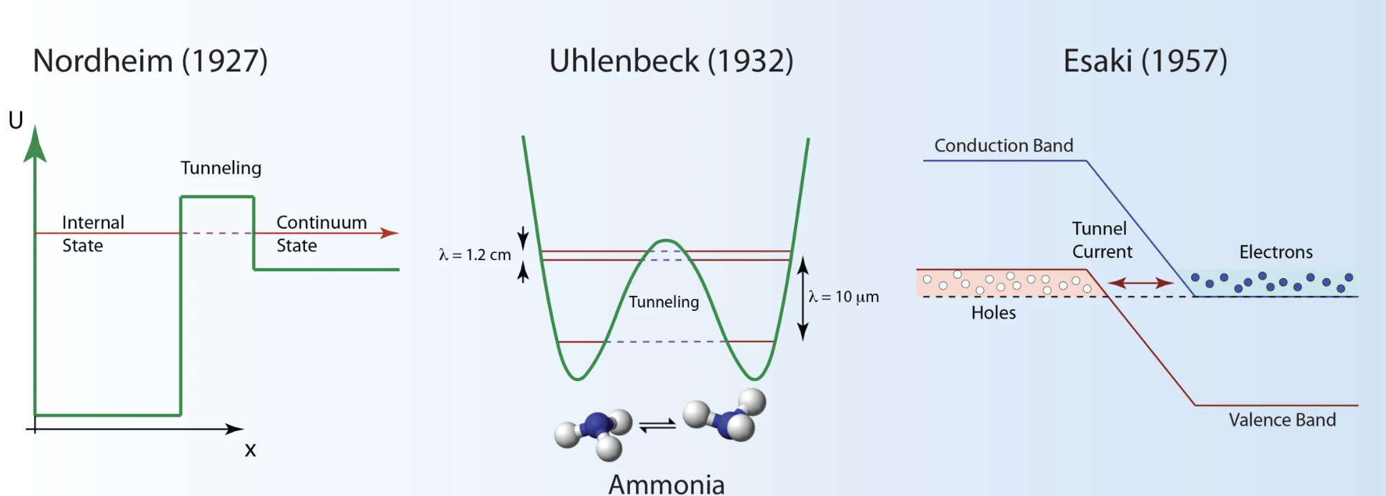
Figure 2:Three early successes of tunneling. Left: electrons escaping a metal through a square barrier (Nordheim, 1927). Middle: inversion of ammonia through the barrier of its double well (Uhlenbeck, 1932). Right: the tunnel diode, in which electrons and holes tunnel across a p-n junction about 10 nm wide (Esaki, 1957).
Alpha decay. An alpha particle trapped in a nucleus tunnels out through the Coulomb barrier (Gamow, and independently Gurney and Condon, 1928). Because is exponential, small differences in energy change half-lives by many orders of magnitude.
Field emission. A strong electric field tilts the barrier at a metal surface, and electrons tunnel out into the vacuum (Fowler and Nordheim, 1928). Field-emission tips are the bright electron sources of modern electron microscopes.
Electronics. Tunnel diodes (Esaki, Nobel Prize 1973), the leakage through ever thinner insulating layers in transistors, and flash memory, which stores each bit by tunneling electrons through an oxide layer.
Chemistry and biology. Long-range electron transfer in photosynthesis and respiration, and hydrogen tunneling in enzymes.
Problems
Problem 1: Penetration depth
An electron in a molecule has an energy 3 eV below the top of the surrounding barrier. (a) Find its penetration depth. (b) By what factor has fallen 2 Å into the barrier? (c) Repeat (a) for a hydrogen atom, about 1837 electron masses.
Solution
Problem 2: How many bound states?
(a) How many bound states does an electron have in a well 1 eV deep and 10 Å wide? (b) What is the smallest depth for which a well 2 Å wide holds a second state?
Solution
Problem 3: A shallow well always binds
Show that the even condition , with , has a solution for every , however small. For find the energy and the penetration depth of this state, and describe what it looks like.
Solution
On the curve rises continuously from 0 to infinity, while the circle starts at and falls. The difference changes sign, so they cross: there is always an even solution.
For small the crossing is at small , where . Then , or , so to leading order
The level sits just below the rim. Its decay constant is , so the penetration depth is far larger than the well itself. A weak well holds its one state loosely: a wide, faint cloud with most of its probability outside.
Problem 4: Through a barrier
An electron with eV meets a barrier 2 eV high and 5 Å wide. (a) Compute from the exact formula. (b) Compare with the thick-barrier approximation. (c) How does change if the width is doubled?
Solution
Here and .
(a) , and , so
(b) , within 2% of the exact value even though is only 2.56.
(c) At 10 Å, and , so : 165 times smaller, close to the factor from the exponential alone.
Problem 5: Reading an STM
An STM tip with eV passes over a feature and the current drops to half. How much farther from the tip is the surface there?
Solution
With and ,
Halving the current takes only a third of an ångström, which is why an STM sees atoms.
Problem 6: An effective box length
The ground state of an electron in the well 5 eV deep and 10 Å wide lies at 0.272 eV. Find its penetration depth, then treat the well as an infinite box widened by one penetration depth on each side, . Compare with the exact energy and with the infinite-box value .
Problem 7: Counting states with the slider
Use the finite-well slider to find the smallest depth at which a well 10 Å wide holds three bound states. Check your answer with , then compare that depth with the levels of an infinite box of the same width. What pattern do you see?
Problem 8: The isotope effect
For a barrier 0.3 eV above the energy and 0.4 Å wide, compute , and their ratio. Which change makes the ratio grow faster: doubling the width, or doubling the height of the barrier above the energy?
Problem 9: Electron transfer in proteins
Rates of electron transfer between redox centers in proteins fall with distance roughly as , with . If the protein acts as a square barrier, what barrier height does this decay constant correspond to? Compare your answer with the energy needed to remove an electron from an organic molecule, about 8 to 10 eV, and suggest why the two differ.
Problem 10: Ammonia and its isotopes
The inversion splitting of NH₃ is 0.79 cm⁻¹ and that of ND₃ is 0.053 cm⁻¹. (a) Convert each splitting to a frequency and to a period . (b) The splitting is roughly proportional to the tunneling amplitude , not to its square. Assuming the umbrella motion’s effective mass doubles from NH₃ to ND₃, use the ratio of the two splittings to estimate for NH₃.
- Cruzeiro, V. W. D., Gao, X., & Kleiman, V. D. (2019). Implementing New Educational Platforms in the Classroom: An Interactive Approach to the Particle in a Box Problem. Journal of Chemical Education, 96(8), 1663–1670. 10.1021/acs.jchemed.9b00195