Operators 2: Hermitian Operators and Commutators

What you need to know

Every observable is a Hermitian operator, $\hat{A}^\dagger = \hat{A}$ : the matrix version of a real number. A Hermitian matrix equals its own mirror image across the diagonal, after its entries are conjugated.
Hermitian operators have real eigenvalues and orthogonal eigenfunctions that form a complete basis: exactly what a measurement needs. For a $2\times 2$ matrix the quadratic formula shows the first property directly.
Momentum $-i\hbar\,d/dx$ is Hermitian because of its $i$ : the derivative alone has imaginary eigenvalues.
Operators need not commute. The commutator $[\hat{A},\hat{B}] = \hat{A}\hat{B} - \hat{B}\hat{A}$ measures the difference between the two orders, and for position and momentum it is never zero: $[\hat{x},\hat{p}] = i\hbar$ .
Operators that commute share their eigenfunctions, so their observables can have sharp values at the same time. Position and momentum cannot.

Operators 1 turned functions into vectors and operators into matrices. This lecture answers the two questions it left open: which matrices may stand for something we can measure, and what happens when two of them do not commute. Both answers are properties of matrices.

Hermitian operators¶

The matrix version of a real number¶

A complex number has a conjugate: flip the sign of $i$ , $(3 + 2i)^* = 3 - 2i$ . A number is real when it equals its own conjugate.
A matrix has an adjoint, written $A^\dagger$ : swap rows and columns, then conjugate every entry, $(A^\dagger)_{jk} = A_{kj}^*$ . A matrix is Hermitian when it equals its own adjoint.

numbers	matrices
conjugate $z^*$ : flip the sign of $i$	adjoint $A^\dagger$ : swap rows and columns, then conjugate
real: $z^* = z$	Hermitian: $A^\dagger = A$

# synced: real_vs_hermitian
import numpy as np
import matplotlib.pyplot as plt
from matplotlib.animation import FuncAnimation
from IPython.display import HTML

TEAL, CARDINAL, GRAY, PURPLE, ORANGE = "#107895", "#C8102E", "#6c757d", "#6a3d9a", "#e07b00"
from matplotlib.patches import Rectangle, FancyArrowPatch
plt.rcParams.update({"axes.spines.top": False, "axes.spines.right": False})
fig, (a1, a2) = plt.subplots(1, 2, figsize=(10.4, 3.9), gridspec_kw={"width_ratios": [1, 1.25], "wspace": 0.12})
a1.axhline(0, color=GRAY, lw=1.8, zorder=1); a1.axvline(0, color=GRAY, lw=0.8, zorder=1)  # a number: the real axis is the mirror
a1.text(5.2, 0.15, "real axis = mirror", color=GRAY, fontsize=12, ha="right", va="bottom")
a1.annotate("", xy=(3, -1.75), xytext=(3, 1.75), arrowprops=dict(arrowstyle="<->", color=GRAY, lw=1.4, ls=(0, (3, 2))))
a1.plot(3, 2, "o", color=TEAL, ms=12, zorder=3); a1.text(3.3, 2, r"$z = 3 + 2i$", color=TEAL, fontsize=15, va="center")
a1.plot(3, -2, "o", color=CARDINAL, ms=12, zorder=3); a1.text(3.3, -2, r"$z^* = 3 - 2i$", color=CARDINAL, fontsize=15, va="center")
a1.plot(1.2, 0, "o", color=PURPLE, ms=12, zorder=3)
a1.text(1.2, -0.5, r"real: $w^* = w$", color=PURPLE, fontsize=14, ha="center", va="top")
a1.set_xlim(-0.4, 5.6); a1.set_ylim(-2.7, 2.7); a1.axis("off")
s0 = 1.25                                                   # a matrix: the diagonal is the mirror
for r in range(2):
    for c in range(2):
        a2.add_patch(Rectangle((c * s0, (1 - r) * s0), s0, s0, fc="#f1ecf7" if r == c else "white", ec=GRAY, lw=1.2, zorder=1))
a2.plot([-0.15, 2 * s0 + 0.15], [2 * s0 + 0.15, -0.15], color=PURPLE, lw=1.6, ls=(0, (4, 3)), zorder=2)
for (xc, yc, lab, col, bg) in ((0.5, 1.5, r"$2$", PURPLE, "#f1ecf7"), (1.5, 0.5, r"$3$", PURPLE, "#f1ecf7"),
                               (1.55, 1.68, r"$1 - i$", TEAL, "white"), (0.45, 0.32, r"$1 + i$", CARDINAL, "white")):
    a2.text(xc * s0, yc * s0, lab, color=col, fontsize=17, ha="center", va="center", zorder=4,
            bbox=dict(boxstyle="round,pad=0.15", fc=bg, ec="none"))
a2.add_patch(FancyArrowPatch((1.36 * s0, 1.36 * s0), (0.64 * s0, 0.64 * s0), arrowstyle="<->", mutation_scale=16,
                             color=GRAY, lw=1.5, zorder=3))
a2.text(2 * s0 + 0.35, 1.75 * s0, "diagonal: on the mirror,\nso it must be real", color=PURPLE, fontsize=13, va="center")
a2.text(2 * s0 + 0.35, 0.95 * s0, r"partners: $(1 - i)^* = 1 + i$", color="k", fontsize=13, va="center")
a2.text(2 * s0 + 0.35, 0.3 * s0, r"$A^\dagger = A$:  Hermitian", color="k", fontsize=15, va="center")
a2.set_xlim(-0.3, 6.4); a2.set_ylim(-0.5, 2 * s0 + 0.3); a2.set_aspect("equal"); a2.axis("off")
fig.text(0.01, 0.95, "a number: conjugate = mirror in the real axis", fontsize=13.5, va="top")
fig.text(0.47, 0.95, "a matrix: mirror in the diagonal, then conjugate", fontsize=13.5, va="top")
fig.subplots_adjust(left=0.01, right=0.99, top=0.86, bottom=0.03)
plt.show()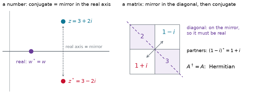

Fig. Left: conjugation mirrors a complex number in the real axis, and a real number sits on the mirror. Right: the adjoint mirrors a matrix in its diagonal and conjugates the entries. In a Hermitian matrix every entry’s mirror partner is its conjugate, and the diagonal entries, which sit on the mirror, must be real.

The adjoint of an operator¶

For an operator, the adjoint $\hat{A}^\dagger$ is whatever you get by moving $\hat{A}$ from the ket to the bra of an inner product:

\langle \phi \vert \hat{A}\psi \rangle = \langle \hat{A}^\dagger\phi \vert \psi \rangle

(1)

For a matrix this is the rule above: swap rows and columns, then conjugate, $(A^\dagger)_{jk} = A_{kj}^*$ . An operator that moves across unchanged is Hermitian, or self-adjoint.

The three grid matrices at the end of Operators 1 are Hermitian. Position and energy are real and symmetric. Momentum is imaginary and antisymmetric: transposing flips the sign of every entry and conjugating flips it back.

Example: which matrices are Hermitian?

A = \begin{pmatrix} 2 & 1-i \\ 1+i & 3 \end{pmatrix}, \quad B = \begin{pmatrix} 1 & 2 \\ 3 & 4 \end{pmatrix}, \quad C = \begin{pmatrix} i & 0 \\ 0 & 1 \end{pmatrix}, \quad D = \begin{pmatrix} 0 & -i \\ i & 0 \end{pmatrix}

(3)

Compare each entry with the conjugate of its mirror image across the diagonal.

$A$ : $A_{12} = 1 - i$ and $A_{21}^* = (1+i)^* = 1 - i$ , and the diagonal is real. Hermitian.
$B$ : $B_{12} = 2$ but $B_{21}^* = 3$ . Not Hermitian.
$C$ : a diagonal entry is its own mirror image, so it must equal its own conjugate, but $i \neq -i$ . A Hermitian matrix has a real diagonal. Not Hermitian.
$D$ : $D_{12} = -i$ and $D_{21}^* = i^* = -i$ . Hermitian, although every off-diagonal entry is imaginary: the same pattern as $\hat{p}$ on the grid.

Why observables must be Hermitian¶

A measurement needs three things from its operator, and Hermitian operators deliver all three.

Real eigenvalues. The eigenvalues are the values a measurement can return, and measured values are real numbers.
Orthogonal eigenfunctions. Eigenfunctions with different eigenvalues satisfy $\langle \phi_m \vert \phi_n \rangle = 0$ : distinct outcomes are mutually exclusive.
A complete basis. Every state can be written as a sum of the eigenfunctions, so every state has a definite probability for each outcome. That is the subject of Measurement.

Example: real eigenvalues from the quadratic formula

Every Hermitian $2\times 2$ matrix has the form $\begin{pmatrix} a & b \\ b^* & d \end{pmatrix}$ with $a$ and $d$ real. Its eigenvalues solve

(a - \lambda)(d - \lambda) - b\,b^* = 0 \quad\Longrightarrow\quad \lambda = \frac{a + d}{2} \pm \sqrt{\Big(\frac{a - d}{2}\Big)^2 + \lvert b\rvert^2}

(5)

Under the square root sits a sum of squares, which is never negative, so both eigenvalues are real. For the matrix $A$ of the previous example, $\lambda = \tfrac{5}{2} \pm \sqrt{\tfrac{1}{4} + 2} = 4$ and 1. The coupling $\lvert b\rvert$ also pushes the two eigenvalues apart, which is why the bonding and antibonding orbitals of ethylene split evenly around the orbital energy (Operators 1, Problem 3).

Proof: the eigenvalues are real

Let $\hat{A}\phi = a\phi$ with $\phi$ normalized. Use the Hermitian property with both functions equal to $\phi$ :

\langle \phi \vert \hat{A}\phi \rangle = a\,\langle \phi \vert \phi \rangle = a, \qquad \langle \hat{A}\phi \vert \phi \rangle = a^*\,\langle \phi \vert \phi \rangle = a^*

(6)

The bra conjugates the constant it carries. Hermitian means the two are equal, so $a = a^*$ .

Proof: eigenfunctions with different eigenvalues are orthogonal

Let $\hat{A}\phi_m = a_m\phi_m$ and $\hat{A}\phi_n = a_n\phi_n$ with $a_m \neq a_n$ . Both eigenvalues are real. Move $\hat{A}$ across the inner product:

\langle \phi_m \vert \hat{A}\phi_n \rangle = a_n\,\langle \phi_m \vert \phi_n \rangle, \qquad \langle \hat{A}\phi_m \vert \phi_n \rangle = a_m\,\langle \phi_m \vert \phi_n \rangle

(7)

The two are equal, so $(a_n - a_m)\,\langle \phi_m \vert \phi_n \rangle = 0$ , and since $a_n \neq a_m$ the overlap vanishes. When several eigenfunctions share one eigenvalue (degeneracy) the argument says nothing, but they can always be combined into orthogonal ones.

The orthogonality is easy to see in the plane:

# synced: eigen_directions
import numpy as np
import matplotlib.pyplot as plt
from matplotlib.animation import FuncAnimation
from IPython.display import HTML

TEAL, CARDINAL, GRAY, PURPLE, ORANGE = "#107895", "#C8102E", "#6c757d", "#6a3d9a", "#e07b00"
plt.rcParams.update({"axes.spines.top": False, "axes.spines.right": False})
t = np.linspace(0, 2 * np.pi, 400); circ = np.array([np.cos(t), np.sin(t)])
arrow = lambda ax, tip, col, lw: ax.annotate("", xy=tip, xytext=(0, 0), arrowprops=dict(
    arrowstyle="-|>", color=col, lw=lw, mutation_scale=16, shrinkA=0, shrinkB=0))
mats = [(np.array([[2.0, 1.0], [1.0, 2.0]]), r"$\binom{2\ \ 1}{1\ \ 2}$", "symmetric"),
        (np.array([[1.0, 1.0], [0.0, 2.0]]), r"$\binom{1\ \ 1}{0\ \ 2}$", "not symmetric"),
        (np.array([[0.0, 1.0], [-1.0, 0.0]]), r"$\left(\genfrac{}{}{0}{}{\ \ 0\quad 1}{-1\ \ \ 0}\right)$", "a rotation")]   # = the two-point d/dx = FS
notes = ["eigen-directions at 90°", "eigen-directions at 45°", "every arrow turns 90° clockwise:\nno eigen-direction"]
fig, axs = plt.subplots(1, 3, figsize=(9.6, 3.9))
for k, (ax, (M, lab, title)) in enumerate(zip(axs, mats)):
    ax.plot(*circ, color=GRAY, lw=1, ls=":")
    ax.axhline(0, color=GRAY, lw=0.6); ax.axvline(0, color=GRAY, lw=0.6)
    w, V = np.linalg.eig(M)
    if k < 2:
        for j in range(2):
            d = V[:, j].real / np.linalg.norm(V[:, j].real); d = d if d[0] >= 0 else -d
            ax.plot([-2.6 * d[0], 2.6 * d[0]], [-2.6 * d[1], 2.6 * d[1]], color=TEAL, lw=2.4, ls="--")
            ax.text(*(2.75 * d), rf"$\lambda = {w[j].real:.0f}$", color=TEAL, fontsize=13,
                    ha="left", va="bottom" if d[1] >= 0 else "top")
    else:
        for deg in (20, 235):                                # turned clockwise to 290 and 145 degrees, clear of the originals
            vv = 1.6 * np.array([np.cos(np.radians(deg)), np.sin(np.radians(deg))])
            arrow(ax, vv, TEAL, 2.6); arrow(ax, M @ vv, CARDINAL, 2.6)
            arc = np.radians(np.linspace(deg - 8, deg - 80, 30))
            ax.plot(0.75 * np.cos(arc), 0.75 * np.sin(arc), color=CARDINAL, lw=1.3)
            ax.annotate("", xy=(0.75 * np.cos(np.radians(deg - 86)), 0.75 * np.sin(np.radians(deg - 86))),
                        xytext=(0.75 * np.cos(arc[-1]), 0.75 * np.sin(arc[-1])),
                        arrowprops=dict(arrowstyle="-|>", color=CARDINAL, lw=1.3, mutation_scale=12))
    ax.set_xlim(-2.9, 3.6); ax.set_ylim(-2.9, 2.9); ax.set_aspect("equal"); ax.axis("off")
    ax.set_title(title, fontsize=14.5)
    ax.text(0.0, 0.98, lab, transform=ax.transAxes, fontsize=15, va="top")
    ax.text(0.5, -0.02, notes[k], transform=ax.transAxes, fontsize=13, ha="center", va="top",
            color=CARDINAL if k == 2 else "k")
fig.subplots_adjust(left=0.01, right=0.99, top=0.9, bottom=0.17, wspace=0.08)
plt.show()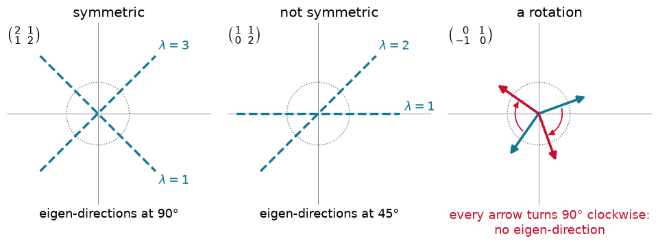

Fig. Eigen-directions of three $2\times 2$ matrices. A symmetric (real Hermitian) matrix has perpendicular eigen-directions. A matrix that is not symmetric can still have real eigenvalues, but its eigen-directions are skewed, here 45° apart. A rotation turns every arrow, so no direction survives and the eigenvalues are complex.

Try the three matrices yourself. For each one, hunt for the eigen-directions or sweep $\mathbf{v}$ once around the circle, and read off the angle between the directions you find.

What goes wrong without Hermiticity? Take a Hermitian matrix and add a growing non-Hermitian part:

# synced: hermitian_dial
import numpy as np
import matplotlib.pyplot as plt
from matplotlib.animation import FuncAnimation
from IPython.display import HTML

TEAL, CARDINAL, GRAY, PURPLE, ORANGE = "#107895", "#C8102E", "#6c757d", "#6a3d9a", "#e07b00"
from matplotlib.colors import LinearSegmentedColormap
plt.rcParams.update({"axes.spines.top": False, "axes.spines.right": False})
wt = LinearSegmentedColormap.from_list("wt", ["white", TEAL])
rng = np.random.default_rng(3)
N = 8
A = rng.normal(size=(N, N)) + 1j * rng.normal(size=(N, N))
Hm, K = (A + A.conj().T) / 2, (A - A.conj().T) / 2           # Hermitian part plus anti-Hermitian part
ss = np.concatenate([np.zeros(5), np.linspace(0, 1, 30), np.ones(6)])
vals, ovl = [], []
for s in ss:
    w, V = np.linalg.eig(Hm + s * K)
    o = np.argsort(w.real)
    V = V[:, o] / np.linalg.norm(V[:, o], axis=0)
    vals.append(w[o]); ovl.append(np.abs(V.conj().T @ V))
allv = np.concatenate(vals)
fig, (ax, axo) = plt.subplots(1, 2, figsize=(8, 3.6), gridspec_kw={"width_ratios": [1.55, 1], "wspace": 0.25})
ax.axhline(0, color=GRAY, lw=1.2)
ax.text(allv.real.max() + 0.2, 0.15, "real axis", color=GRAY, fontsize=11, ha="right", va="bottom")
scat = ax.scatter(vals[0].real, vals[0].imag, s=70, color=TEAL, zorder=5)
ax.set_xlim(allv.real.min() - 0.5, allv.real.max() + 0.5)
lim = 1.15 * max(0.5, np.abs(allv.imag).max())
ax.set_ylim(-lim, lim)
ax.set_xlabel("Re (eigenvalue)", fontsize=12); ax.set_ylabel("Im (eigenvalue)", fontsize=12)
img = axo.imshow(ovl[0], cmap=wt, vmin=0, vmax=1)
axo.set_xticks([]); axo.set_yticks([])
for sp in axo.spines.values():
    sp.set_visible(False)
axo.set_title(r"overlaps $|\langle v_j | v_k \rangle|$", fontsize=13)
fig.subplots_adjust(left=0.09, right=0.98, top=0.84, bottom=0.15)

def update(i):
    w, s = vals[i], ss[i]
    scat.set_offsets(np.column_stack([w.real, w.imag]))
    scat.set_color([TEAL if abs(v.imag) < 1e-6 else CARDINAL for v in w])
    img.set_data(ovl[i])
    off = (ovl[i] - np.diag(np.diag(ovl[i]))).max()
    ax.set_title(rf"$A = H + s\,K$,  $s = {s:.2f}$:  " + ("eigenvalues real" if s == 0 else f"largest |Im| = {np.abs(w.imag).max():.2f}"),
                 loc="left", fontsize=12.5)
    axo.set_xlabel("eigenvectors orthonormal" if s == 0 else f"largest overlap {off:.2f}", fontsize=12)

ani = FuncAnimation(fig, update, frames=len(ss), interval=110, blit=False)
plt.close(fig)
HTML(ani.to_jshtml())

Fig. A Hermitian matrix $H$ ( $s = 0$ ) has real eigenvalues (left, all on the real axis) and orthonormal eigenvectors, so their overlaps (right) form the identity. Adding $s$ times a non-Hermitian part $K$ , with $K^\dagger = -K$ , pushes the eigenvalues into the complex plane, and the eigenvectors start to overlap. Neither could describe a measurement.

Hermitian is more than “real eigenvalues”. The matrix $\begin{pmatrix} 1 & 1 \\ 0 & 2 \end{pmatrix}$ has the real eigenvalues 1 and 2, but its eigenvectors overlap (Problem 4). Its outcomes would not be mutually exclusive, so it cannot represent an observable.

Momentum and its $i$ ¶

Example: the derivative on two points

On two grid points, with $\psi = 0$ beyond the ends, the derivative matrix is $D_1 = \frac{1}{2\Delta x}\begin{pmatrix} 0 & 1 \\ -1 & 0 \end{pmatrix}$ . It turns every arrow by 90°, like the rotation in the figure above, so no direction survives and its eigenvalues are imaginary:

\det(D_1 - \lambda I) = \lambda^2 + \frac{1}{4\Delta x^2} = 0 \quad\Longrightarrow\quad \lambda = \pm\frac{i}{2\Delta x}

(8)

Multiplying by $-i\hbar$ gives the momentum matrix and real eigenvalues:

P = -i\hbar D_1 = \frac{\hbar}{2\Delta x}\begin{pmatrix} 0 & -i \\ i & 0 \end{pmatrix}, \qquad p = \pm\frac{\hbar}{2\Delta x}

(9)

$P$ is $\tfrac{\hbar}{2\Delta x}$ times the Hermitian matrix $D$ of the example above. The factor $-i$ in $\hat{p} = -i\hbar\,d/dx$ turns the imaginary eigenvalues of the derivative into real momenta. The grid derivative of a plane wave in Operators 1 showed the same on a large grid: eigenvalue $i\sin(k\Delta x)/\Delta x$ , made real by $-i\hbar$ .

Example: is momentum Hermitian?

Integrate by parts. The boundary term vanishes because physical wavefunctions go to zero at infinity, or at the walls of a box:

\int_{-\infty}^{\infty}\phi^*\left(-i\hbar\frac{d\psi}{dx}\right)dx = \Big[-i\hbar\,\phi^*\psi\Big]_{-\infty}^{\infty} + i\hbar\int_{-\infty}^{\infty}\frac{d\phi^*}{dx}\,\psi\,dx = \int_{-\infty}^{\infty}\left(-i\hbar\frac{d\phi}{dx}\right)^{\!*}\psi\,dx

(10)

The last step uses $\big(-i\hbar\,\phi'\big)^* = i\hbar\,\phi'^*$ . So $\langle \phi \vert \hat{p}\psi \rangle = \langle \hat{p}\phi \vert \psi \rangle$ : momentum is Hermitian.

Without the $i$ it fails. The same steps give $\int\phi^*\psi'\,dx = -\int(\phi')^*\psi\,dx$ , so $d/dx$ is anti-Hermitian, $(d/dx)^\dagger = -d/dx$ . The factor $-i$ turns the minus sign around, which is why momentum carries an $i$ .

Commutators: the order of operations¶

Order matters¶

$\hat{A}\hat{B}\psi$ means: apply $\hat{B}$ first, then $\hat{A}$ . For numbers the order never matters, $3 \times 5 = 5 \times 3$ . For operators, as for matrices, it often does.

Can two observables be sharp at once?¶

A state with a sharp value $a$ of an observable is an eigenfunction, $\hat{A}\psi = a\psi$ . Sharp values of two observables at once need $\hat{B}\psi = b\psi$ as well. Then the order does not matter on that state:

\hat{A}\hat{B}\,\psi = \hat{A}\,(b\psi) = ab\,\psi, \qquad \hat{B}\hat{A}\,\psi = \hat{B}\,(a\psi) = ba\,\psi \qquad\Longrightarrow\qquad \big[\hat{A},\hat{B}\big]\,\psi = 0

(12)

So two observables can be sharp together only on states where their commutator gives zero. When the commutator gives zero on no state at all, as for position and momentum below, no state is sharp in both.

Two matrices that do not commute¶

The matrix $F = \begin{pmatrix} 1 & 0 \\ 0 & -1 \end{pmatrix}$ flips an arrow in the $x$ axis, and $S = \begin{pmatrix} 0 & 1 \\ 1 & 0 \end{pmatrix}$ swaps its two components, a mirror in the line $y = x$ . Applied one after the other, the order decides the result:

# synced: flip_swap
import numpy as np
import matplotlib.pyplot as plt
from matplotlib.animation import FuncAnimation
from IPython.display import HTML

TEAL, CARDINAL, GRAY, PURPLE, ORANGE = "#107895", "#C8102E", "#6c757d", "#6a3d9a", "#e07b00"
from matplotlib.patches import FancyArrowPatch
plt.rcParams.update({"axes.spines.top": False, "axes.spines.right": False})
F = np.array([[1.0, 0.0], [0.0, -1.0]])                    # flip: mirror in the x axis
S = np.array([[0.0, 1.0], [1.0, 0.0]])                     # swap: mirror in the line y = x
strokes = [np.array([[0.25, 0.2], [0.25, 1.0]]), np.array([[0.25, 1.0], [0.8, 1.0]]),
           np.array([[0.25, 0.6], [0.65, 0.6]])]          # the letter F, each stroke as rows [x, y]
draw = lambda ax, M, col, lw, ls, alpha: [ax.plot(*(M @ s.T), color=col, lw=lw, ls=ls, alpha=alpha,
                                                  solid_capstyle="round") for s in strokes]
fig, axs = plt.subplots(1, 3, figsize=(9.6, 3.7))
panels = [(None, None, "start", ""),
          (S, F @ S, r"swap, then flip:  $F\,S$", "turned 90° clockwise"),
          (F, S @ F, r"flip, then swap:  $S\,F$", "turned 90° counterclockwise")]
for ax, (M1, M2, title, note) in zip(axs, panels):
    ax.axhline(0, color=GRAY, lw=0.8); ax.axvline(0, color=GRAY, lw=0.8)
    draw(ax, np.eye(2), TEAL, 7, "-", 1.0 if M1 is None else 0.3)
    if M1 is not None:
        draw(ax, M1, GRAY, 3.5, (0, (1.5, 2.5)), 0.8)      # after the first step
        draw(ax, M2, CARDINAL, 7, "-", 1.0)                 # after both steps
    ax.set_xlim(-1.5, 1.5); ax.set_ylim(-1.5, 1.5); ax.set_aspect("equal"); ax.axis("off")
    ax.set_title(title, fontsize=14.5)
    ax.text(0.5, -0.02, note, transform=ax.transAxes, fontsize=13, ha="center", va="top", color=CARDINAL)
for ax, (a0, a1) in ((axs[1], (78, -12)), (axs[2], (72, 162))):   # the net turn, drawn outside the letters
    arc = np.radians(np.linspace(a0, a1, 60))
    ax.plot(1.38 * np.cos(arc), 1.38 * np.sin(arc), color=CARDINAL, lw=1.6)
    ax.add_patch(FancyArrowPatch((1.38 * np.cos(arc[-4]), 1.38 * np.sin(arc[-4])), (1.38 * np.cos(arc[-1]), 1.38 * np.sin(arc[-1])),
                                 arrowstyle="-|>", mutation_scale=18, color=CARDINAL, lw=1.6))
fig.subplots_adjust(left=0.01, right=0.99, top=0.88, bottom=0.12, wspace=0.08)
plt.show()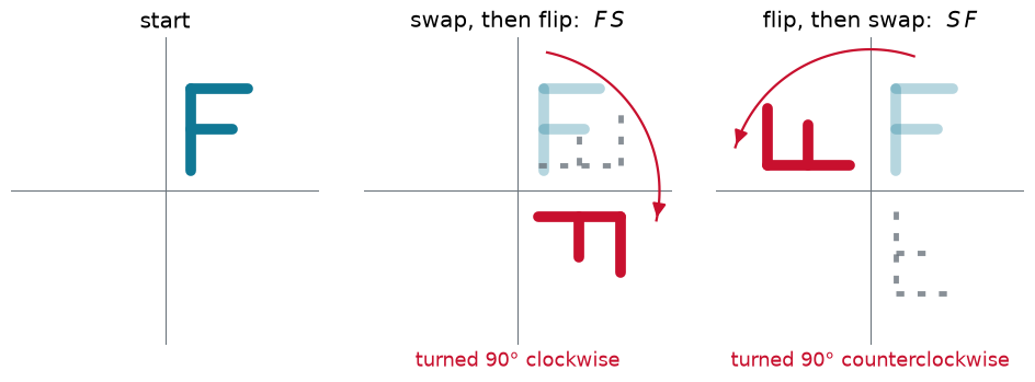

Fig. The letter F mirrored twice. Swapping first and then flipping ( $FS$ ) turns it 90° clockwise; flipping first and then swapping ( $SF$ ) turns it 90° counterclockwise. Same two steps, opposite results.

FS = \begin{pmatrix} 0 & 1 \\ -1 & 0 \end{pmatrix}, \qquad SF = \begin{pmatrix} 0 & -1 \\ 1 & 0 \end{pmatrix}, \qquad [F, S] = \begin{pmatrix} 0 & 2 \\ -2 & 0 \end{pmatrix} \neq 0

(13)

Try it: press F and S in either order and watch the letter turn over each mirror. The panel keeps the product of the matrices, written right to left like operators. Play both orders to see the two results side by side, then try F twice, or F S twice.

Both matrices are Hermitian, so both could stand for observables, yet they do not commute, and they share no eigenvector: $F$ keeps $(1, 0)$ and $(0, 1)$ , while $S$ keeps $(1, \pm 1)$ . These two matrices measure the spin of an electron along $z$ and along $x$ (Spin); Operators as Matrices works the same product in its Problem 3.

Position and momentum¶

The recipe for any commutator of differential operators: act on a test function $f$ , use the product rule, and drop $f$ at the end.
Multiply by $-i\hbar$ and the example becomes the most important commutator in quantum mechanics:

Example: $XP - PX$ on three grid points

On three points spaced $\Delta x$ apart, $X = \operatorname{diag}(x_1, x_2, x_3)$ , and the momentum matrix $P = -i\hbar D_1$ has $-i\hbar/2\Delta x$ just above the diagonal and $+i\hbar/2\Delta x$ just below it. Entry by entry, $(XP)_{jk} = x_j P_{jk}$ and $(PX)_{jk} = P_{jk}\,x_k$ , so

(XP - PX)_{jk} = (x_j - x_k)\,P_{jk}

(17)

Only neighbors survive, and they differ by $x_j - x_{j\pm 1} = \mp\Delta x$ , which cancels the $1/2\Delta x$ in $P$ :

XP - PX = \frac{i\hbar}{2}\begin{pmatrix} 0 & 1 & 0 \\ 1 & 0 & 1 \\ 0 & 1 & 0 \end{pmatrix}

(18)

Acting on a vector, this matrix replaces each value by $i\hbar$ times the average of its two neighbors. For a smooth function that average is close to the value itself, so $(XP - PX)\,\psi \approx i\hbar\,\psi$ : the canonical commutator, as accurate as the grid.

With many points, numpy confirms it. Build $C = XP - PX$ on 400 points and apply it to a smooth function:

import numpy as np

N = 400; x = np.linspace(-8, 8, N); dx = x[1] - x[0]
X = np.diag(x)
P = -1j * (np.eye(N, k=1) - np.eye(N, k=-1)) / (2 * dx)     # hbar = 1
C = X @ P - P @ X

psi = np.exp(-x**2 / 2) * (1 + 0.3 * x)                     # any smooth function
print(f"largest |C psi - i psi|: {np.abs(C @ psi - 1j * psi)[5:-5].max():.1e}")
print("largest diagonal entry of C:", np.abs(np.diag(C)).max())

largest |C psi - i psi|: 9.0e-04
largest diagonal entry of C: 0.0

$C\psi$ matches $i\psi$ to about 10^-3, the accuracy of the grid, yet the diagonal of $C$ is zero. That is no accident:

Why no finite matrices can obey $[X, P] = i\hbar$ exactly

You might expect $C = XP - PX$ to be $i\hbar$ times the identity matrix. It cannot be. The trace of a product does not depend on the order, $\operatorname{tr}(XP) = \operatorname{tr}(PX)$ , so $\operatorname{tr} C = 0$ , while $\operatorname{tr}(i\hbar\,I) = i\hbar N$ . No pair of $N \times N$ matrices satisfies the canonical commutator; only operators on infinitely many dimensions can.

Rules for commutators¶

An operator commutes with itself and its powers: $[\hat{A},\hat{A}] = [\hat{A},\hat{A}^n] = 0$ . So $[\hat{p},\hat{K}] = [\hat{p}, \hat{p}^2/2m] = 0$ .
Swapping the order flips the sign: $[\hat{A},\hat{B}] = -[\hat{B},\hat{A}]$ , so $[\hat{p},\hat{x}] = -i\hbar$ .
Functions of $x$ commute with each other: $[\hat{x}, V(x)] = 0$ .
A product rule: $[\hat{A},\hat{B}\hat{C}] = [\hat{A},\hat{B}]\,\hat{C} + \hat{B}\,[\hat{A},\hat{C}]$ (Problem 5).

Example: momentum and energy of a free particle

For a free particle $V = 0$ and $\hat{H} = \hat{p}^2/2m$ . Is the plane wave $e^{ikx}$ an eigenfunction of $\hat{p}$ ? Of $\hat{H}$ ?

\hat{p}\,e^{ikx} = -i\hbar\,(ik)\,e^{ikx} = \hbar k\,e^{ikx}, \qquad \hat{H}\,e^{ikx} = \frac{1}{2m}\,\hat{p}\big(\hbar k\,e^{ikx}\big) = \frac{\hbar^2k^2}{2m}\,e^{ikx}

(19)

Yes to both: this state has a sharp momentum and a sharp energy. The two operators commute, $\hat{H}\hat{p} = \hat{p}^3/2m = \hat{p}\hat{H}$ .

The function $\sin kx$ is an eigenfunction of $\hat{H}$ with the same energy but not of $\hat{p}$ (Problem 4 of The Schrödinger Equation). There is no contradiction: $e^{ikx}$ and $e^{-ikx}$ have the same energy, so any mix of them, $\sin kx$ included, is an eigenfunction of $\hat{H}$ . The theorem promises that shared eigenfunctions exist, here the two plane waves, not that every eigenfunction of $\hat{H}$ is one of them.

Why, in three steps. Suppose no other eigenfunction of $\hat{A}$ has the eigenvalue $a$ .

Start from $\hat{A}\phi = a\phi$ .
Swap the order, which is allowed because the operators commute: $\hat{A}\big(\hat{B}\phi\big) = \hat{B}\big(\hat{A}\phi\big) = a\,\big(\hat{B}\phi\big)$ .
So $\hat{B}\phi$ is also an eigenfunction of $\hat{A}$ with the eigenvalue $a$ . The only such function is $\phi$ itself, up to a constant: $\hat{B}\phi = b\,\phi$ .

If several eigenfunctions share an eigenvalue (degeneracy), $\hat{B}$ can mix them, and the shared eigenfunctions are particular combinations, as in the free-particle example above.

The converse: shared eigenfunctions mean the operators commute

Suppose $\hat{A}$ and $\hat{B}$ share a complete set of eigenfunctions, $\hat{A}\phi_n = a_n\phi_n$ and $\hat{B}\phi_n = b_n\phi_n$ . Expand an arbitrary function in that set, $\psi = \sum_n c_n\phi_n$ , and use linearity:

\hat{A}\hat{B}\,\psi = \sum_n c_n\,\hat{A}\big(b_n\phi_n\big) = \sum_n c_n\,a_nb_n\,\phi_n, \qquad \hat{B}\hat{A}\,\psi = \sum_n c_n\,\hat{B}\big(a_n\phi_n\big) = \sum_n c_n\,b_na_n\,\phi_n

(21)

The numbers $a_nb_n$ and $b_na_n$ are equal, so $\hat{A}\hat{B}\psi = \hat{B}\hat{A}\psi$ for every $\psi$ : the operators commute. The argument needs the set to be complete, because the commutator must vanish on every function, not just on a few.

Commuting observables can have sharp values at the same time: a state of definite momentum also has a definite kinetic energy. Position and momentum do not commute, and no state has sharp values of both. Measurement turns this into the uncertainty principle.
The labels of chemistry are shared eigenvalues. The quantum numbers $n$ , $l$ , $m$ of a hydrogen orbital label simultaneous eigenfunctions of three commuting operators, $\hat{H}$ , $\hat{L}^2$ and $\hat{L}_z$ (Chapter 5).
The translation table of Operators 1 gains two rows:

	integral	Dirac	numpy on a grid
adjoint	$\int (\hat{A}^\dagger\phi)^\,\psi\,dx = \int \phi^\,\hat{A}\psi\,dx$	$\hat{A}^\dagger$	`A.conj().T`
commutator	$\hat{A}\hat{B}\psi - \hat{B}\hat{A}\psi$	$[\hat{A},\hat{B}]$	`A @ B - B @ A`

Problems¶

Problem 1: Complete the Hermitian matrix¶

Fill in the missing entries so that each matrix is Hermitian, or explain why it cannot be done:

A = \begin{pmatrix} 4 & 2 - 3i \\ \square & -1 \end{pmatrix}, \qquad B = \begin{pmatrix} \square & 5i \\ \square & 0 \end{pmatrix}, \qquad C = \begin{pmatrix} 1 & \square \\ 7 & 2i \end{pmatrix}, \qquad D = \begin{pmatrix} 0 & \square & 1 \\ i & 3 & \square \\ \square & 4 & 2 \end{pmatrix}

(22)

Solution

Every off-diagonal entry must be the conjugate of its mirror partner, and every diagonal entry must be real.

$A$ : the missing entry is $A_{21} = A_{12}^* = 2 + 3i$ .
$B$ : $B_{21} = (5i)^* = -5i$ , and $B_{11}$ can be any real number.
$C$ : impossible. The diagonal entry $2i$ is not real, whatever goes in the blank (which would have to be 7).
$D$ : $D_{12} = D_{21}^* = -i$ , $D_{23} = D_{32}^* = 4$ and $D_{31} = D_{13}^* = 1$ .

Problem 2: The parity operator¶

The parity operator reflects a function through the origin, $\hat{\Pi}f(x) = f(-x)$ . Show that $\hat{\Pi}$ is Hermitian, and find its eigenvalues and eigenfunctions. Which states of the finite square well of Tunneling and the Finite Square Well are eigenfunctions of $\hat{\Pi}$ ?

Solution

Hermitian. Substitute $y = -x$ , which maps the interval $(-\infty, \infty)$ onto itself:

\int_{-\infty}^{\infty}\phi^*(x)\,\psi(-x)\,dx = \int_{-\infty}^{\infty}\phi^*(-y)\,\psi(y)\,dy = \int_{-\infty}^{\infty}\big(\hat{\Pi}\phi\big)^*\,\psi\,dy

(23)

Eigenvalues. Reflecting twice gives back the function, $\hat{\Pi}^2 f = f$ . If $\hat{\Pi}f = \lambda f$ then $\hat{\Pi}^2f = \lambda^2 f = f$ , so $\lambda^2 = 1$ and $\lambda = \pm 1$ , real as promised. The eigenfunctions with $\lambda = +1$ are the even functions, $f(-x) = f(x)$ , and those with $\lambda = -1$ the odd ones.

The well. The bound states of the finite well came out even (cosines inside) or odd (sines inside), so each is an eigenfunction of $\hat{\Pi}$ . That is the shared-eigenfunction theorem at work: when $V(-x) = V(x)$ , $\hat{\Pi}$ commutes with $\hat{H}$ , and the stationary states can be chosen to have definite parity.

Problem 3: Momentum on a four-point grid¶

Build the $4\times4$ momentum matrix on a periodic grid of four points with spacing $\Delta x$ , using the centered difference and $\hbar = 1$ (on a periodic grid the neighbors of point 1 are points 4 and 2). Show that it is Hermitian and find its eigenvalues.

Solution

Row $j$ of the derivative matrix holds $+1/2\Delta x$ for the right neighbor and $-1/2\Delta x$ for the left one, wrapping around at the ends. Multiplying by $-i$ :

P = \frac{-i}{2\Delta x}\begin{pmatrix} 0 & 1 & 0 & -1 \\ -1 & 0 & 1 & 0 \\ 0 & -1 & 0 & 1 \\ 1 & 0 & -1 & 0 \end{pmatrix}

(24)

The real matrix in parentheses is antisymmetric ( $d/dx$ is anti-Hermitian). For $P$ , compare $P_{12} = -i/2\Delta x$ with $P_{21}^* = (+i/2\Delta x)^* = -i/2\Delta x$ : equal, and likewise for every pair, with zeros on the diagonal. $P$ is Hermitian.

import numpy as np
dx = 1.0
M = np.array([[0, 1, 0, -1], [-1, 0, 1, 0], [0, -1, 0, 1], [1, 0, -1, 0]])
P = -1j * M / (2 * dx)
print(np.allclose(P, P.conj().T))           # True
print(np.round(np.linalg.eigvalsh(P), 6))   # [-1.  0.  0.  1.]

The eigenvalues $-1/\Delta x, 0, 0, +1/\Delta x$ are real, and the eigenvectors are discrete plane waves $e^{ikx_j}$ : the grid version of the momentum eigenfunctions.

Problem 4: Real eigenvalues are not enough¶

Find the eigenvalues and normalized eigenvectors of $M = \begin{pmatrix} 1 & 1 \\ 0 & 2 \end{pmatrix}$ and the overlap between the eigenvectors. Could $M$ represent an observable?

Solution

$M$ is triangular, so its eigenvalues are the diagonal entries, 1 and 2: both real. The eigenvectors are

\lambda = 1:\ \mathbf{v}_1 = \begin{pmatrix}1\\0\end{pmatrix}, \qquad \lambda = 2:\ \mathbf{v}_2 = \frac{1}{\sqrt{2}}\begin{pmatrix}1\\1\end{pmatrix}, \qquad \langle \mathbf{v}_1 \vert \mathbf{v}_2 \rangle = \frac{1}{\sqrt{2}} \neq 0

(25)

$M$ is not Hermitian ( $M_{12} = 1$ but $M_{21} = 0$ ), and the price is overlapping eigenvectors. A system in state $\mathbf{v}_2$ would have a nonzero overlap with the outcome “1”, although it is supposed to give “2” with certainty. The outcomes are not mutually exclusive, so $M$ cannot represent an observable.

Problem 5: Commutator algebra¶

Prove the product rule $[\hat{A},\hat{B}\hat{C}] = [\hat{A},\hat{B}]\,\hat{C} + \hat{B}\,[\hat{A},\hat{C}]$ by expanding both sides. Use it, with $[\hat{x},\hat{p}] = i\hbar$ , to find $[\hat{x},\hat{p}^3]$ and $[\hat{x}^2,\hat{p}]$ .

Problem 6: Momentum and force¶

Show that $[\hat{p}, V(x)] = -i\hbar\,\dfrac{dV}{dx}$ by acting on a test function. Evaluate it for a particle on a spring, $V = \tfrac{1}{2}kx^2$ , and for a uniform field, $V = mgx$ . For which potentials does $\hat{p}$ commute with $\hat{H}$ ?

Problem 7: Why centered differences?¶

Instead of the centered difference, approximate the derivative by the forward difference $\psi'(x_j) \approx (\psi_{j+1} - \psi_j)/\Delta x$ . Write the $3\times 3$ forward-difference matrix $D_f$ for three points with $\psi = 0$ beyond the ends, and the momentum matrix $P_f = -i\hbar D_f$ . Is $P_f$ Hermitian? Find its eigenvalues (the matrix is triangular). What would a measurement of this “momentum” return, and what does that say about the choice of the centered difference?

Problem 8: Building a shared eigenfunction¶

For a free particle, show that $\cos kx$ is an eigenfunction of $\hat{H}$ but not of $\hat{p}$ . Which combinations $a\cos kx + b\sin kx$ are eigenfunctions of both, and what are their momenta?

Hermitian operators¶

The matrix version of a real number¶

The adjoint of an operator¶

Why observables must be Hermitian¶

Momentum and its iii¶

Commutators: the order of operations¶

Order matters¶

Can two observables be sharp at once?¶

Two matrices that do not commute¶

Position and momentum¶

Rules for commutators¶

Commuting operators share eigenfunctions¶

Problems¶

Problem 1: Complete the Hermitian matrix¶

Problem 2: The parity operator¶

Problem 3: Momentum on a four-point grid¶

Problem 4: Real eigenvalues are not enough¶

Problem 5: Commutator algebra¶

Problem 6: Momentum and force¶

Problem 7: Why centered differences?¶

Problem 8: Building a shared eigenfunction¶

Momentum and its $i$ ¶