Acknowledgement
These Jupyter notebooks are based on the excellent paper in J. Chem. Educ. 2019, 96, 8, 1663-1670.
Quantum objects can go where no classical particles are allowed!
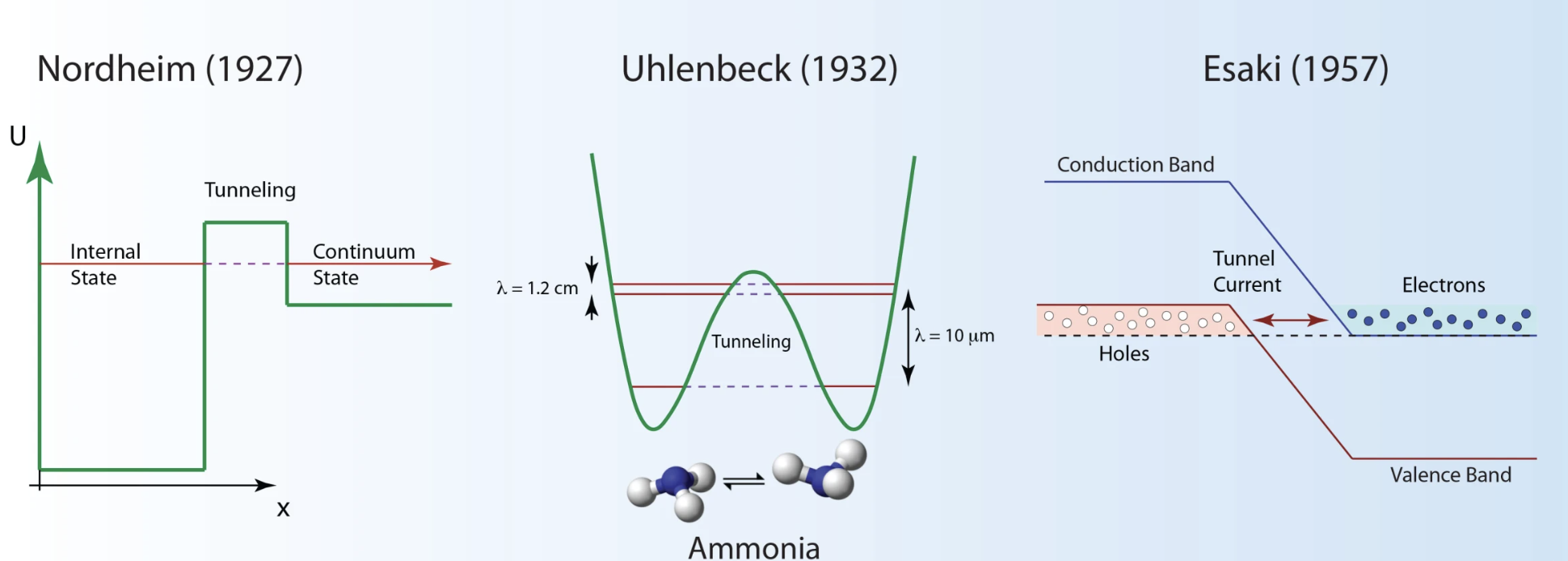
Figure 1:Nordheim square barrier for electron tunneling from bound states into the continuum.
Nitrogen inversion in ammonia by tunneling through the barrier (proposed by George Uhlenbeck in 1932).
Esaki tunnel diode: electrons and holes tunnel across a heavily doped p-n junction only about 10 nm wide.
Qualitative trends in wavefunction behavior
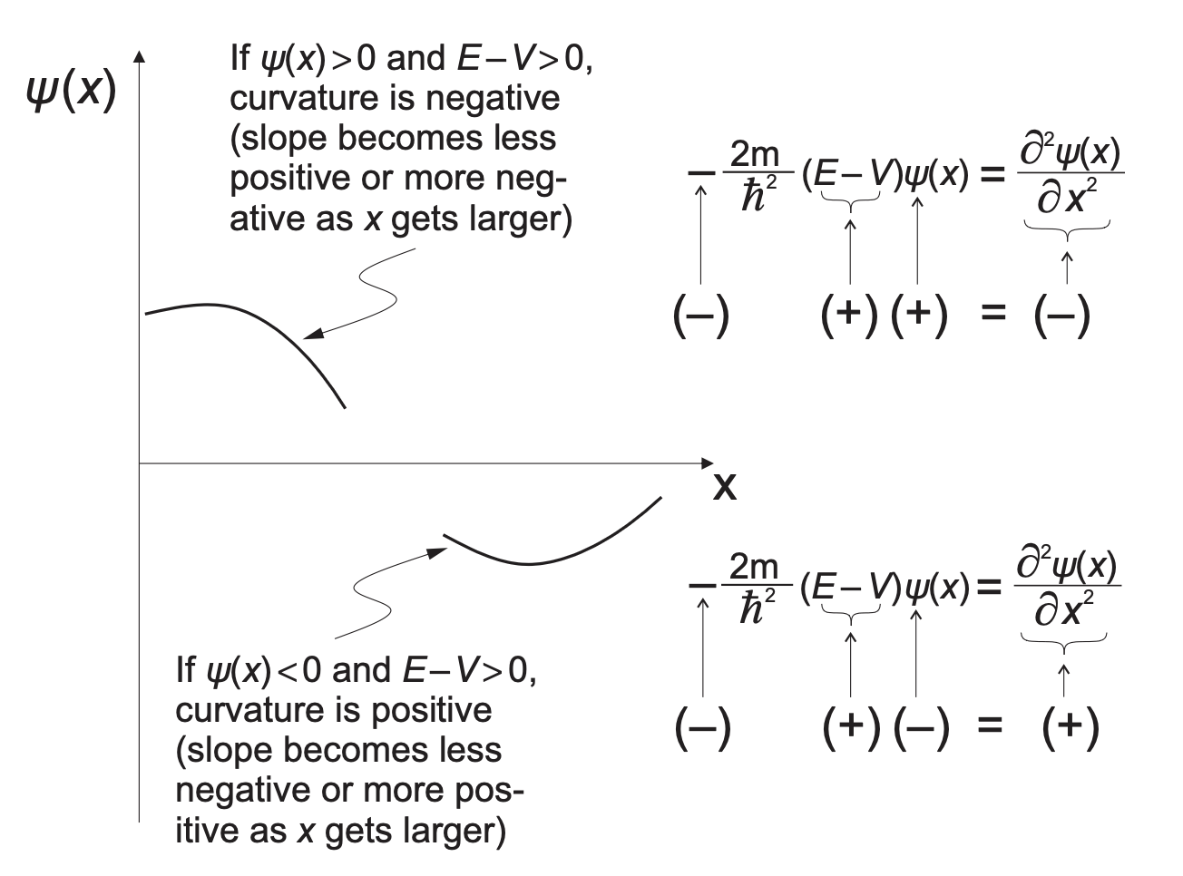
Figure 2:A stepped potential and the expected behavior of the wavefunction.
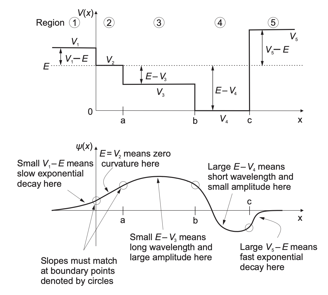
Figure 3:From the signs of the terms in the Schrödinger equation, we can predict qualitatively how the wavefunction will behave.
Source
###############################################################################################
#
#  The cell contains all of the libraries used in the notebook, either run all cells or
#  execute the cells in order starting with this.
#
#  In google colab run all is ctrl+F8 or select "run all" from the runtime menu above
#
###############################################################################################

import matplotlib as mpl # matplotlib library for plotting and visualization
import matplotlib.pylab as plt # matplotlib library for plotting and visualization
import numpy as np #numpy library for numerical manipulation, especially suited for data arrays
import matplotlib.patches as mpatches
from matplotlib.lines import Line2D
from scipy import optimize

import warnings
warnings.filterwarnings('ignore')

#widget modules, to allow interaction with plots
from ipywidgets import interactive
import ipywidgets as widgets
#IPython for interactive outputs from cells
from IPython.display import display, HTML, Image, Markdown

#To animate the 3D plots and produce movies
from matplotlib import animation
from mpl_toolkits.mplot3d import Axes3D

#Use to test the system, different response from some code
#depending on whether the notebook is being compiled into a webpage,
#run in jupyter or in google colab.
import sys
import psutil

IN_COLAB = 'google.colab' in sys.modules
PARENT_PROC = psutil.Process().parent().cmdline()[-1]

#set variable to identify the environment for execution.
if 'jupyter-lab' in PARENT_PROC:
    interactive_env = True
elif 'jupyter-notebook' in PARENT_PROC:
    interactive_env = True
elif IN_COLAB:
    interactive_env = True
else:
    interactive_env = False
#function to produce complex number from Euler form.
def P2R(radii, angles):
    return radii * np.exp(1j*angles)

#constants used later
hbar = 1.05457180013e-34 # planck's constant divided by 2*pi, in Joules*second
melec = 9.10938356e-31 # mass of an electron in kg
eVtoJ = 1.60217662e-19 # conversion factor from eV to Joules
AngstromtoMeter = 1e-10 # conversion factor from Angstroms to meters
val = np.sqrt(2.0*melec*eVtoJ)*AngstromtoMeter/(2.0*hbar) # prefactor sqrt(2*melec)/(2*hbar), for when L is in angstroms and Vo is in eV

#####


fig_no = 1
def potential(x, Vo, L):
    Vx=np.zeros(len(x))
    for i in range(len(x)):
        if x[i]<=-L/2 or x[i]>=L/2:
            Vx[i]=Vo


    return Vx

L=10
Vo=5

fig, ax=plt.subplots()

#create and plot the potential
x = np.linspace(-L, L, 1000)
Vx = potential(x, Vo, L)
ax.plot(x,Vx, label='Potential $V_0$')

ax.set_ylim(-.1,Vo*1.4)
ax.set_xlim(-L,L)
ax.set_xlabel(r'$x$ (Angstroms)', fontsize=14)
ax.set_ylabel(r'Energy (eV)', fontsize=14);

#label the three regions of the potential
ax.annotate('Region I',xy=(-3*L/4,Vo*1.1), ha='center')
ax.annotate('Region II',xy=(0,Vo*1.1), ha='center')
ax.annotate('Region III',xy=(3*L/4,Vo*1.1), ha='center')

#generic plot, label interms of width L and depth Vo
ax.set_yticks([0, Vo])
ax.set_yticklabels(['0','$V_0$'])
ax.set_xticks([-L/2, L/2])
ax.set_xticklabels(['$-L/2$','$L/2$'])

#highlight the classically forbidden region in gray
ax.bar(-3*L/4, Vo, width=L/2, color='gray', alpha=0.5)
ax.bar(3*L/4, Vo, width=L/2, color='gray', alpha=0.5)
ax.bar(0, -0.1, width=2*L, color='gray', alpha=0.5)

patch = mpatches.Patch(color='gray', label='Classically forbidden region')
handles, labels = ax.get_legend_handles_labels()
handles.append(patch)
ax.legend(handles=handles, loc=2);

plt.show()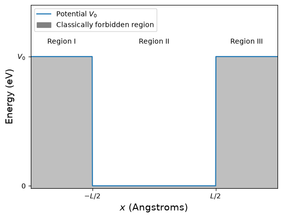
Solutions inside square well
Inside the finite square well, the region , the potential so the Schrödinger equation,
Solutions to this equation have an oscillatory form:
Solutions outside the well
In the regions where and , the potential is . The time-independent Schrödinger equation for these regions can be written as:
where . The value of differs in each region of the well depending on the energy and the potential.
What happens when ?
When the particle’s energy is less than the potential outside the well , the term becomes negative. This makes positive, so is real and the solution in this region is an exponential decay (an evanescent wave). The wavefunction therefore decays exponentially as the particle penetrates into the classically forbidden regions outside the well.
Profile of the full wavefunction
Our potential well consists of three regions, and the particle has an energy less than the potential, i.e. . So that the wavefunction can be normalized, we make the following choices to ensure that as . We also choose the trigonometric form of the wavefunction inside the well; recall that this is to make the math easier.
Why do we check for continuity?
needs to be continuous to guarantee the existence of , whose existence is required from the first postulate.
is a component of the kinetic energy operator. If the wavefunction does not have a well-defined second derivative, then the kinetic energy would be undefined, which is not possible.
Boundary conditions
The wavefunction is the combination of all three components, so we make sure that the wavefunction and its first derivative are continuous at each boundary. We apply the following boundary conditions to achieve this:
Note that there are two conditions at each boundary, so we end up with two sets of two simultaneous equations.
Even and odd solutions
Finally, our potential is symmetric about , so the wavefunction is either a maximum or zero at so that the probability distribution is symmetric about . We call these even when and odd when .
Even solutions:
These are called even solutions because the function is even, i.e. it is symmetric about . However, they correspond to the odd values of .
After imposing the boundary conditions we reach the following relation:
Odd solutions:
These are called odd solutions because the function is odd, i.e. it is anti-symmetric about . However, they correspond to the even values of . This is a bit confusing, I know, but the labeling of is arbitrary; the sine and cosine solutions themselves are determined by the physics.
After imposing the boundary conditions we reach the following relation:
Unfortunately, we cannot find the allowed energies analytically. Instead, we have to choose either a graphical or a numerical method.
What does that mean? We can graph the left- and right-hand sides of each equation separately as a function of energy and look for the intersection points, which correspond to the allowed energy values (the energy eigenvalues).
Below, the functions for the odd and even wavefunctions are plotted using the Desmos graphing tool. You can adjust the potential and the length , and you can click on the intercept points to read off the energy and the value of the function.
Finding the energy eigenvalues graphically
Source
#a better (tidier!!) way of finding the energy eigen values in the finite square well.

#define the equations we wish to find the roots of
#one for even wavefuntions and one for odd wavefunctions.

def f_even(E,Vo,L):
    return(np.sqrt(Vo-E)-np.sqrt(E)*np.tan(L*np.sqrt(E)*val))
def f_odd(E,Vo,L):
    return(np.sqrt(Vo-E)+np.sqrt(E)/np.tan(L*np.sqrt(E)*val))

#function to find the roots of the above equations.
#default step size of 0.04 is sufficient given the well
#parameters being used in the rest of the notebook.

def find_state_energies(Vo,L,step=0.01):

    sol = np.array([],dtype=float) #all solutions
    E = np.arange(step,Vo,step) #array of energies
    even=True

    #iterate over the array of energies and look for positions where the sign of the function changes
    #These are the roots of the function.
    for i in range(len(E)-1):
        if even==True:
            if f_even(E[i], Vo, L)*f_even(E[i+1], Vo, L)<0: #have we bracketed a zero?
                sol=np.append(sol,optimize.brentq(f_even,E[i],E[i+1],args=(Vo, L)) )
                even=False
        if even==False:
            if f_odd(E[i], Vo, L)*f_odd(E[i+1], Vo, L)<0:
                sol=np.append(sol,optimize.brentq(f_odd,E[i],E[i+1],args=(Vo, L)))
                even=True
    #return the energies of the states and the number of states
    return sol, len(sol)

#eng, nstates = sqWellSol(5, 10)
#print(eng, nstates)
#print(e_eng)
Source
# plot the odd and even solutions, identify the intercepts with an energy label.

def solve_finite_square_well(Vo, L):
    # Generating the graph
    fig, axes = plt.subplots(1, 2, figsize=(12,6), gridspec_kw={'width_ratios': [2, 1]})
    axes[0].axis([0.0,Vo,0.0,np.sqrt(Vo)*1.1])
    axes[0].set_xlabel(r'$E$ (eV)')
    axes[0].set_ylabel(r'(eV$^{-1}$)')
    E = np.linspace(0.0, Vo, 10000)
    num = int(round((L*np.sqrt(Vo)*val-np.pi/2.0)/np.pi))
    # Removing discontinuity points
    for n in range(10000):
        for m in range(num+2):
            if abs(E[n]-((2.0*float(m)+1.0)*np.pi/(2.0*L*val))**2)<0.01: E[n] = np.nan
            if abs(E[n]-(float(m)*np.pi/(L*val))**2)<0.01: E[n] = np.nan
    # Plotting the curves and setting the labels
    axes[0].plot(E, np.sqrt(Vo-E), label=r"$\sqrt{V_o-E}$", color="blue", linewidth=1.8)
    axes[0].plot(E, np.sqrt(E)*np.tan(L*np.sqrt(E)*val), label=r"Even states: $\sqrt{E}\tan(\frac{L\sqrt{2mE}}{2\hbar})$", color="red", linestyle='-.', linewidth=1.8)
    axes[0].plot(E, -np.sqrt(E)/np.tan(L*np.sqrt(E)*val), label=r"Odd states: $-\frac{\sqrt{E}}{\tan(\frac{L\sqrt{2mE}}{2\hbar})}$", color="green", linestyle='--', linewidth=1.8)
    axes[0].legend(loc=1, borderaxespad=0.0)

    energies, nstates = find_state_energies(Vo, L)
    ydata = np.sqrt(Vo-energies)
    axes[0].scatter(energies[:nstates], ydata[:nstates])
    state = 0
    for i,j in zip(energies[:nstates],ydata[:nstates]):
        state+=1
        axes[0].annotate('$E_{%d} = $%.3f eV' %(state, i), xy=(i,j), textcoords='offset points')
    ##draw energy levels
    axes[1].spines['right'].set_color('none')
    axes[1].yaxis.tick_left()
    axes[1].spines['bottom'].set_color('none')
    axes[1].axes.get_xaxis().set_visible(False)
    axes[1].spines['top'].set_color('none')
    axes[1].axis([-15,15,0.0,10])
    axes[1].set_ylabel(r'$E_n$ (eV)')

    for n in range(0,nstates):
        str1="$n = "+str(n+1)+r"$, $E_"+str(n+1)+r" = %.3f$ eV"%(energies[n])
        if (n+1)%2:
            statecolour = 'red'
            stateline = '-.'
        else:
            statecolour = 'green'
            stateline = '--'
        axes[1].text(1.1*L/2, energies[n]-0.005*Vo, str1, fontsize=12, color=statecolour)
        axes[1].hlines(energies[n], -L/2, L/2, linewidth=1.8, linestyle=stateline, color=statecolour)

    #plot the potential
    x = np.linspace(-15,15,1000)
    Vx = potential(x, Vo, L)
    axes[1].plot(x,Vx, color='blue',linewidth=1.5)

    # Show the plots on the screen once the code reaches this point
    plt.show()

Llabel = r"Vo"
nlabel = r"L"
interactive_plot = widgets.interactive(solve_finite_square_well,Vo=widgets.FloatSlider(min=0.1, max=10, step=0.5, value=5, description=Llabel,orientation='horizontal'),
                               L=widgets.FloatSlider(min=0.1, max=17, step=0.1, value=10, description=nlabel,orientation='horizontal'))
display(interactive_plot)
#create some figure information
#figstring = 'Figure 2.6.'+str(fig_no)+': On the left are the solutions to the left and right hand size of equation. On the right is the energy level diagram.'
#fig_no+=1
#display(Markdown(figstring))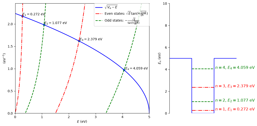
Here are some questions to think about:
Q1: How does changing the width affect the number and energy of the states?
Q2: How does changing the potential affect the number and energy of the states?
Q3: Is the ground state described by an even or an odd wavefunction?
Q4: What is the minimum number of states?
Q5: Do the energy levels follow the same pattern as the infinite square well, i.e. ?
Plots of the wavefunctions and probability densities
Now that we know the energy eigenvalues, we can use them to find expressions for the wavefunctions and probability densities. This may help you understand some of the choices we made up to this point. Take a look at the figure and consider again the choice of wavefunction in regions I and III, and why we split the wavefunction into odd and even functions inside the well.
Source
#set the potential depth and width
Vo=5
L=10

#find the energies of the states for the given Vo and L
E_vals, nstates = find_state_energies(Vo, L)

fig, ax = plt.subplots(1,2, figsize=(12,9))

#create x values for each of region I, II & III
X_lef = np.linspace(-L, -L/2.0, 900,endpoint=True)
X_mid = np.linspace(-L/2.0, L/2.0, 900,endpoint=True)
X_rig = np.linspace(L/2.0, L, 900,endpoint=True)

#set some figure parameters
ax[0].axis([-L,L,0.0,1.2*Vo])
ax[0].set_xlabel(r'$X$ (Angstroms)')
ax[0].set_ylabel(r'$\psi(x)$')

# Define the maximum amplitude of the wavefunction
if (nstates > 1):
    amp = np.sqrt((E_vals[1]-E_vals[0])/1.5)
else:
    amp = np.sqrt((Vo-E_vals[0])/1.5)

# Plot the wavefunctions
for n in range(1,nstates+1):
    ax[0].hlines(E_vals[n-1], -L, L, linewidth=1.8, linestyle='--', color="black")
    k = 2.0*np.sqrt(E_vals[n-1])*val
    a0 = 2.0*np.sqrt(Vo-E_vals[n-1])*val
    # Plotting odd wavefunction
    if (n%2==0):
        ax[0].plot(X_lef,E_vals[n-1]-amp*np.exp(a0*L/2.0)*np.sin(k*L/2.0)*np.exp(a0*X_lef), color="red", label="", linewidth=2.8)
        ax[0].plot(X_mid,E_vals[n-1]+amp*np.sin(k*X_mid), color="red", label="", linewidth=2.8)
        ax[0].plot(X_rig,E_vals[n-1]+amp*np.exp(a0*L/2.0)*np.sin(k*L/2.0)*np.exp(-a0*X_rig), color="red", label="", linewidth=2.8)
    # Plot even wavefunction
    else:
        ax[0].plot(X_lef,E_vals[n-1]+amp*np.exp(a0*L/2.0)*np.cos(k*L/2.0)*np.exp(a0*X_lef), color="red", label="", linewidth=2.8)
        ax[0].plot(X_mid,E_vals[n-1]+amp*np.cos(k*X_mid), color="red", label="", linewidth=2.8)
        ax[0].plot(X_rig,E_vals[n-1]+amp*np.exp(a0*L/2.0)*np.cos(k*L/2.0)*np.exp(-a0*X_rig), color="red", label="", linewidth=2.8)

#create the potential
x = np.linspace(-L,L,1000)
Vx = potential(x, Vo, L)
ax[0].plot(x,Vx, color='blue',linewidth=1.5)

#create a legend
handles, labels = ax[0].get_legend_handles_labels()
line = Line2D([0], [0], label='Wavefunction $\psi(x)$', color='red', linestyle='-')
handles.append(line)
line = Line2D([0], [0], label='Energy Level $E_n$', color='black', linestyle='--')
handles.append(line)
line = Line2D([0], [0], label='Potential $V_0$', color='blue', linestyle='-')
handles.append(line)
ax[0].legend(handles=handles, loc=2);

#start plotting the probability densities
#axis properties for probability densities
ax[1].axis([-L,L,0.0,1.2*Vo])
ax[1].set_xlabel(r'$x$ (Angstroms)')
ax[1].set_ylabel(r'$|\psi(x)|^2$')

#Label the potential
str1="$V_o = %.3f$ eV"%(Vo)
ax[1].text(1.1*L, 1.02*Vo, str1, fontsize=14, color="blue")

# Defining the maximum amplitude of the probability density
if (nstates > 1):
    amp = (E_vals[1]-E_vals[0])/1.5
else:
    amp = (Vo-E_vals[0])/1.5

# Plot the probability densities
for n in range(1,nstates+1):
    ax[1].hlines(E_vals[n-1], -L, L, linewidth=1.8, linestyle='--', color="black")
    str1="$n = "+str(n)+r"$, $E_"+str(n)+r" = %.3f$ eV"%(E_vals[n-1])
    ax[1].text(1.1*L, E_vals[n-1]+0.01*Vo, str1, fontsize=12, color="red")
    k = 2.0*np.sqrt(E_vals[n-1])*val
    a0 = 2.0*np.sqrt(Vo-E_vals[n-1])*val
    # Plot odd probability densities
    if (n%2==0):
        Y_lef = E_vals[n-1]+amp*(np.exp(a0*L/2.0)*np.sin(k*L/2.0)*np.exp(a0*X_lef))**2
        ax[1].plot(X_lef,Y_lef, color="red", linewidth=2.8)
        ax[1].fill_between(X_lef, E_vals[n-1], Y_lef, color="green", alpha=0.7)
        ax[1].plot(X_mid,E_vals[n-1]+amp*(np.sin(k*X_mid))**2, color="red", label="", linewidth=2.8)
        Y_rig = E_vals[n-1]+amp*(np.exp(a0*L/2.0)*np.sin(k*L/2.0)*np.exp(-a0*X_rig))**2
        ax[1].plot(X_rig,Y_rig, color="red", linewidth=2.8)
        ax[1].fill_between(X_rig, E_vals[n-1], Y_rig, color="green", alpha=0.7)
    # Plot even probability densities
    else:
        Y_lef = E_vals[n-1]+amp*(np.exp(a0*L/2.0)*np.cos(k*L/2.0)*np.exp(a0*X_lef))**2
        ax[1].plot(X_lef,Y_lef, color="red", linewidth=2.8)
        ax[1].fill_between(X_lef, E_vals[n-1], Y_lef, color="green", alpha=0.7)
        ax[1].plot(X_mid,E_vals[n-1]+amp*(np.cos(k*X_mid))**2, color="red", label="", linewidth=2.8)
        Y_rig = E_vals[n-1]+amp*(np.exp(a0*L/2.0)*np.cos(k*L/2.0)*np.exp(-a0*X_rig))**2
        ax[1].plot(X_rig,Y_rig, color="red", linewidth=2.8)
        ax[1].fill_between(X_rig, E_vals[n-1], Y_rig, color="green", alpha=0.7)


#create a legend
handles, labels = ax[1].get_legend_handles_labels()
line = Line2D([0], [0], label='Probability Density $|\psi(x)|^2$', color='red', linestyle='-')
handles.append(line)
line = Line2D([0], [0], label='Energy Level $E_n$', color='black', linestyle='--')
handles.append(line)
line = Line2D([0], [0], label='Potential $V_0$', color='blue', linestyle='-')
handles.append(line)
patch = mpatches.Patch(color='green', alpha=0.7, label='Probability of being in \nclassically forbidden region')
handles.append(patch)
ax[1].legend(handles=handles, loc=2);

ax[1].plot(x,Vx, color='blue',linewidth=1.5)

plt.show()

plt.show()


#figstring = 'Figure 2.6.'+str(fig_no)+': label.'
#fig_no+=1
#display(Markdown(figstring))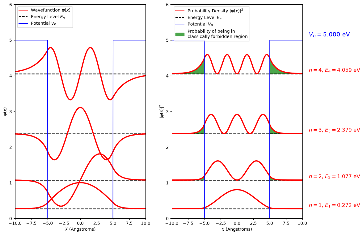
From these plots we can explain some of the behaviour of the energy levels as and are changed.
The first thing to note from the diagram above is that the wavefunctions extend outside the potential; they enter what is sometimes called the classically forbidden region.
As with the potential step, the quantum description of the particle allows it to tunnel into a region where the potential is larger than the energy of the particle. This is indicated by the shaded green area in the probability density plot. Note that this area gets larger as approaches zero.
Tunneling of particle in the box
The tunneling probability corresponds to the area outside the box that has non-zero probability density. In the graphical representation, those areas are shaded green. Integrating over those areas gives the probability that the particle tunnels outside the classically allowed region.
We can calculate , i.e. the size of the shaded green area as a percentage of the total area:
Source
#@title  { vertical-output: true, form-width: "60%", display-mode: "form" }
print ("\nThe tunneling probabilities are:")
for n in range(1,nstates+1):
    k = 2.0*np.sqrt(E_vals[n-1])*val
    a0 = 2.0*np.sqrt(Vo-E_vals[n-1])*val
    # For odd solution
    if (n%2==0):
        C = 1.0
        D = np.exp(a0*L/2.0)*np.sin(k*L/2.0)*C
        prob = D*D*2.0*k*np.exp(-a0*L)/(B*B*a0*(k*L-np.sin(k*L))+D*D*2.0*k*np.exp(-a0*L))
    # For even solution
    else:
        B = 1.0
        D = np.exp(a0*L/2.0)*np.cos(k*L/2.0)*B
        prob = D*D*2.0*k*np.exp(-a0*L)/(B*B*a0*(k*L+np.sin(k*L))+D*D*2.0*k*np.exp(-a0*L))
    print("  State #%3d tunneling probability = %5.2f%%" % (n,100*prob))
The tunneling probabilities are:
  State #  1 tunneling probability =  0.83%
  State #  2 tunneling probability =  3.55%
  State #  3 tunneling probability =  9.25%
  State #  4 tunneling probability = 23.30%
A comparison between the energies of an infinite and a finite square well
These values confirm what we have already deduced: the closer the state is to the top of the potential, the more easily it spreads outside the well. How does this affect the energy levels? Lower in the potential, the wavelength of the wavefunction is more closely tied to the width of the well than it is higher up. Compare the infinite and finite square wells of the same width below.
Source
h=6.62607e-34    #planck's constant in joules
me=9.1093837e-31  # mass of an electron in kg

def En_infinite_square_well(n,L):
    return n**2*h**2/(8*me*(L*1e-10)**2*1.6e-19)

def compare_infinite_and_finite_square_wells(Vo, L):
    # Generating the graph
    fig, axes = plt.subplots(1, 2, figsize=(9,6), layout='constrained')

    nmax = 1
    axes[0].spines['right'].set_color('none')
    axes[0].yaxis.tick_left()
    axes[0].spines['bottom'].set_color('none')
    axes[0].axes.get_xaxis().set_visible(False)
    axes[0].spines['top'].set_color('none')
    axes[0].axis([0.0,10.0,0.0,1.1*Vo])
    axes[0].set_ylabel(r'$E_n$ (eV)')
    while En_infinite_square_well(nmax, L) < Vo:
        str1="$n = "+str(nmax)+r"$, $E_"+str(nmax)+r" = %.3f$ eV"%(En_infinite_square_well(nmax, L))
        if (nmax)%2:
            statecolour = 'red'
        else:
            statecolour = 'green'
        axes[0].text(6.5, En_infinite_square_well(nmax, L), str1, fontsize=12, color=statecolour)
        axes[0].hlines(En_infinite_square_well(nmax, L), 0.0, 6.3, linewidth=1.8, linestyle='--', color=statecolour)
        nmax+=1

    energies, nstates = find_state_energies(Vo, L)
    ydata = np.sqrt(Vo-energies)
    ##draw energy levels
    axes[1].spines['right'].set_color('none')
    axes[1].yaxis.tick_left()
    axes[1].spines['bottom'].set_color('none')
    axes[1].axes.get_xaxis().set_visible(False)
    axes[1].spines['top'].set_color('none')
    axes[1].axis([0.0,10.0,0.0,1.1*Vo])
    axes[1].set_ylabel(r'$E_n$ (eV)')

    for n in range(0,nstates):
        str1="$n = "+str(n+1)+r"$, $E_"+str(n+1)+r" = %.3f$ eV"%(energies[n])
        if (n+1)%2:
            statecolour = 'red'
        else:
            statecolour = 'green'
        axes[1].text(6.5, energies[n]-0.005*Vo, str1, fontsize=12, color=statecolour)
        axes[1].hlines(energies[n], 0.0, 6.3, linewidth=1.8, linestyle='--', color=statecolour)
    str1="$V_o = %.3f$ eV"%(Vo)
    axes[1].text(6.5, Vo-0.01*Vo, str1, fontsize=12, color="blue")
    axes[1].hlines(Vo, 0.0, 6.3, linewidth=2.5, linestyle='-', color="blue")
    axes[1].hlines(0.0, 0.0, 6.3, linewidth=1.2, linestyle='-', color="black")

    plt.show()

Llabel = r"Vo"
nlabel = r"L"
interactive_plot = widgets.interactive(compare_infinite_and_finite_square_wells,Vo=widgets.FloatSlider(min=0.1, max=10, step=0.5, value=5, description=Llabel,orientation='horizontal'),
                               L=widgets.FloatSlider(min=0.1, max=17, step=0.1, value=10, description=nlabel,orientation='horizontal'))
display(interactive_plot)
#figstring = 'Figure: On the left are the are the energy levels in the infinite square well. On the right are the energy levels for the finite square well of the same width but height Vo.'
#display(Markdown(figstring))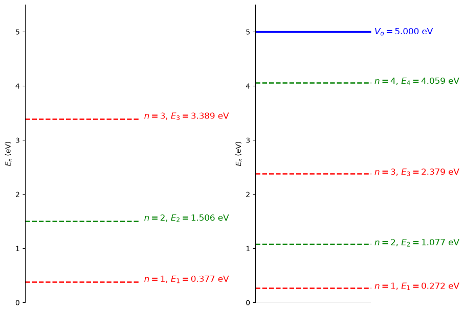
Notice that at energies closer to zero, the infinite and finite energies are closer together. As the energy of the state approaches the top of the finite potential, it is smaller in the finite well than in the infinite well. Why? The higher-energy states allow the wavefunction in the finite square well to spread out, so the wavelength is longer in the finite well than in the infinite well. A longer wavelength corresponds to a smaller wavenumber , and hence a lower energy.
- Cruzeiro, V. W. D., Gao, X., & Kleiman, V. D. (2019). Implementing New Educational Platforms in the Classroom: An Interactive Approach to the Particle in a Box Problem. Journal of Chemical Education, 96(8), 1663–1670. 10.1021/acs.jchemed.9b00195