The Wavefunction

What is the meaning of a wave-function $\psi$ ?¶

• In the classical wave equation, the wave function has a clear mechanical interpretation: it represents the degree of disturbance in the wave. For example, it can describe the elevation of a guitar string from its resting position.

• In contrast, the quantum wave function is less intuitive. The wave function itself does not have direct physical meaning, as it is generally a complex function. To connect it to measurable quantities, we need to extract real values from it that correspond to physical observables.

• The key insight is that the absolute square of the wave function gives the probability distribution:

• $p(x)$ is a probability distribution function. It describes the likelihood of finding a quantum object at a position $x$.

• $p(x)\,dx$ gives the probability of finding the particle in a tiny part of space inside the interval $[x, x+dx]$.

• In three-dimensional space, the analogous expression is:

  $$p(x, y, z) = \psi(x, y, z)^{*} \cdot \psi(x, y, z)$$

  (2)

Probability Refresher¶

• Before introducing quantum mechanics and wavefunctions, let’s recall some core ideas from probability.

Random Variables¶

• A random variable assigns numbers to the outcomes of an experiment. For example, how many squirrels you see each day is a random variable.

• Discrete examples: dice rolls, coin flips.

• Continuous examples: particle position, measurement noise.

Probability Distributions¶

• A continuous random variable is fully described by a distribution over all possible values. We call this object a probability distribution $p(x)$, which must integrate (or sum, in the discrete case) to one, showing that we cover all possibilities and that each possibility is assigned a fraction of 1.

Further Exploration¶

• Video overview

• Interactive probability explorer

Source

import matplotlib.pyplot as plt
import numpy as np

# Discrete probabilities (fair dice)
outcomes = np.arange(1, 7)
probs = np.ones_like(outcomes) / 6

plt.bar(outcomes, probs)
plt.xlabel("Dice outcome")
plt.ylabel("Probability")
plt.title("PMF of a Fair Die")
plt.show()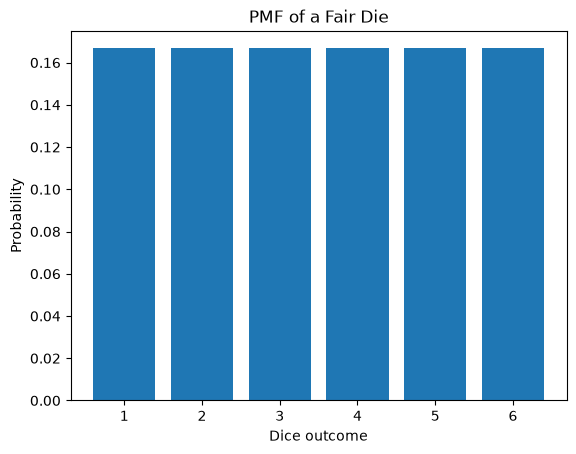

Source

# Continuous uniform distribution on [a,b]
a, b = 0, 1
x = np.linspace(-0.2, 1.2, 200)
pdf = np.where((x >= a) & (x <= b), 1/(b-a), 0)

plt.plot(x, pdf, lw=2)
plt.fill_between(x, pdf, alpha=0.3)
plt.xlabel("x")
plt.ylabel("p(x)")
plt.title("Uniform Distribution on [0,1]")
plt.show()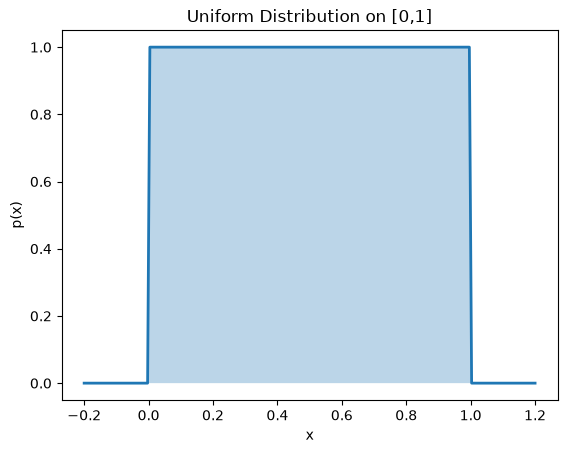

Source

from scipy.stats import norm

x = np.linspace(-4, 4, 200)
pdf = norm.pdf(x, loc=0, scale=1)

plt.plot(x, pdf, label="N(0,1)")
plt.fill_between(x, pdf, alpha=0.2)
plt.xlabel("x")
plt.ylabel("p(x)")
plt.title("Gaussian PDF")
plt.legend()
plt.show()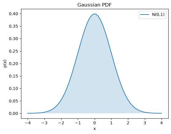

Source

# -----------------------------
# Correct sampling for H-atom 1s
# -----------------------------
N = 6000
a0 = 1.0

# For 1s: if x = 2r/a0, then x ~ Gamma(k=3, theta=1)
x = np.random.gamma(shape=3.0, scale=1.0, size=N)
r = 0.5 * a0 * x

# Isotropic angles
u = np.random.rand(N)
theta = np.arccos(1 - 2*u)
phi = 2*np.pi*np.random.rand(N)

# Convert to Cartesian and take a 2D projection
x3 = r * np.sin(theta) * np.cos(phi)
y3 = r * np.sin(theta) * np.sin(phi)

# Histogram for the shell probability density P(r) (per unit r)
bins = np.linspace(0, 6*a0, 80)
hist, edges = np.histogram(r, bins=bins, density=True)
centers = 0.5*(edges[1:] + edges[:-1])

# Analytical radial distribution P(r) = 4 r^2 |psi|^2 = 4 r^2 / (a0^3*pi) * exp(-2r/a0) * pi
# Simplifies to: P(r) = (4/a0^3) r^2 exp(-2r/a0), which integrates to 1
rr = np.linspace(0, bins[-1], 400)
P_r = (4.0/(a0**3)) * rr**2 * np.exp(-2*rr/a0)

# Side-by-side subplots: dot cloud and radial distribution

fig, axs = plt.subplots(1, 2, figsize=(12, 5))

# Left: simulated dot cloud
axs[0].scatter(x3, y3, s=1, alpha=0.5)
axs[0].set_title("Hydrogen 1s: position observations (2D projection)")
axs[0].set_xlabel("x [$a_0$]")
axs[0].set_ylabel("y [$a_0$]")
axs[0].set_aspect('equal')

# Right: radial distribution histogram + analytical curve
axs[1].plot(centers, hist, lw=2, label="Monte Carlo (histogram)")
axs[1].plot(rr, P_r, lw=2, linestyle="--", label="Analytical 1s")
axs[1].set_title("Radial probability distribution")
axs[1].set_xlabel("r [$a_0$]")
axs[1].set_ylabel("$P(r)$")
axs[1].legend()

plt.tight_layout()
plt.show()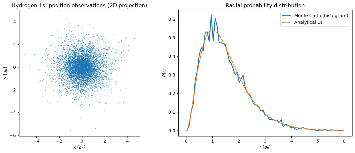

Normalization of wavefunction¶

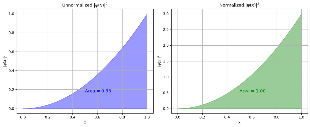
• For the wave function to represent a proper probability distribution, it must be normalizable. If it is not normalizable, the wave function is only proportional to a probability distribution and not equal to it.

• Normalization of $\psi^2$ ensures that there is absolute certainty that the quantum object exists somewhere in space. In an experiment, when searching for a quantum particle across the entire space, normalization guarantees that you will find it somewhere.

• Normalization in 1D:

  $$\int^{+\infty}_{-\infty} |\psi(x)|^2 dx = \int^{+\infty}_{-\infty} p(x) dx = 1$$

  (22)

• To normalize a wave function $\psi'$, multiply it by a constant: $\psi = N\psi'$. The constant $N$ is determined by plugging this expression into the normalization condition. In other words, normalization determines the multiplicative factor in front of the wave function.

• Normalization in 3D:

  $$\int^{+\infty}_{-\infty} \int^{+\infty}_{-\infty} \int^{+\infty}_{-\infty} |\psi(x, y, z)|^2 dx \, dy \, dz = 1$$

  (23)

Source

import numpy as np
import matplotlib.pyplot as plt

# Define x values
x = np.linspace(0, 1, 500)

# Unnormalized psi
psi_unnorm = x
psi2_unnorm = psi_unnorm**2

# Normalized psi (C = sqrt(3))
psi_norm = np.sqrt(3) * x
psi2_norm = psi_norm**2

# Compute integrals for annotation
area_unnorm = np.trapezoid(psi2_unnorm, x)
area_norm = np.trapezoid(psi2_norm, x)

# Create the figure and axes
fig, axes = plt.subplots(1, 2, figsize=(12, 5))

# --- Plot 1: Unnormalized psi² ---
axes[0].fill_between(x, psi2_unnorm, alpha=0.4, color="blue")
axes[0].set_title("Unnormalized $|\psi(x)|^2$")
axes[0].set_xlabel("x")
axes[0].set_ylabel(r"$|\psi(x)|^2$")
axes[0].grid(True)
axes[0].text(0.5, 0.2, rf"Area = {area_unnorm:.2f}", 
             transform=axes[0].transAxes, fontsize=12, color="blue")

# --- Plot 2: Normalized psi² ---
axes[1].fill_between(x, psi2_norm, alpha=0.4, color="green")
axes[1].set_title("Normalized $|\psi(x)|^2$")
axes[1].set_xlabel("x")
axes[1].set_ylabel(r"$|\psi(x)|^2$")
axes[1].grid(True)
axes[1].text(0.5, 0.2, rf"Area = {area_norm:.2f}", 
             transform=axes[1].transAxes, fontsize=12, color="green")

plt.tight_layout()
plt.show()

<>:24: SyntaxWarning: invalid escape sequence '\p'
<>:33: SyntaxWarning: invalid escape sequence '\p'
<>:24: SyntaxWarning: invalid escape sequence '\p'
<>:33: SyntaxWarning: invalid escape sequence '\p'
/tmp/ipykernel_3080/3267431332.py:24: SyntaxWarning: invalid escape sequence '\p'
  axes[0].set_title("Unnormalized $|\psi(x)|^2$")
/tmp/ipykernel_3080/3267431332.py:33: SyntaxWarning: invalid escape sequence '\p'
  axes[1].set_title("Normalized $|\psi(x)|^2$")

What can we do with probability distribution functions (PDF)?¶

• By definition, the probability distribution function $p(x)$ lets us quantify the probability that a quantum “particle” is located in an infinitesimal slice $[x, x+dx]$ around the point $x$. This then enables us to find the probability in any finite region $[a,b]$ simply by integrating:

  $$p(a<x<b)=\int_a^b |\psi(x)|^2dx$$

  (30)

• In higher dimensions, e.g. 3D, we can locate the particle within a volume element $dx\,dy\,dz$, or any finite volume, via a similar integration:

  $$p(a_x<x<b_x,a_y<y<b_y, a_z<z<b_z )=\int^{b_x}_{a_x} \int^{b_y}_{a_y} \int^{b_z}_{a_z} |\psi(x,y,z)|^2dx dy dz$$

  (31)

What about quantities which correspond to operators?¶

• Recall that the mean value of $x$ is computed by weighting its values by their probabilities. For example, think of the average mass of a box of candies: we multiply the probability (or fraction) of each candy type by its mass and sum.

• Likewise, you can compute the average of any function of $x$, say $x^2$ or $\sin(x)$.

• For quantities like momentum or total energy, which are no longer simple functions as in classical mechanics but operators, $\hat{p}$ and $\hat{H}$, we simply use the operators in the definition of the moments:

Source

import numpy as np
import matplotlib.pyplot as plt
from math import erf, sqrt

# ----- Parameters -----
sigma = 1.0  # width of the Gaussian (harmonic oscillator ground state)
x0, x1 = -1.0, 1.0  # interval to integrate over

# ----- Define |psi(x)|^2 for a normalized Gaussian -----
def prob_density(x, sigma):
    # |psi(x)|^2 = (1/(sqrt(2*pi)*sigma)) * exp(-x^2/(2*sigma^2))
    return (1.0/(np.sqrt(2*np.pi)*sigma)) * np.exp(-x**2/(2*sigma**2))

# Probability via the error function (analytic CDF of a normal distribution)
def interval_probability(a, b, sigma):
    return 0.5*(erf(b/(sqrt(2)*sigma)) - erf(a/(sqrt(2)*sigma)))

P = interval_probability(x0, x1, sigma)

# ----- Plot -----
xs = np.linspace(-4*sigma, 4*sigma, 800)
ys = prob_density(xs, sigma)

fig = plt.figure(figsize=(10, 5))

# Title with the integral expression
plt.title(r"$P_{x_0<x<x_1}=\int_{x_0}^{x_1}|\psi(x)|^2\,dx$" + 
          f"\nSelected interval: [{x0:.2f}, {x1:.2f}]",
          loc="left")

# Curve
plt.plot(xs, ys, linewidth=3)

# Shade between x0 and x1 under the curve
mask = (xs >= x0) & (xs <= x1)
plt.fill_between(xs[mask], ys[mask], 0, alpha=0.25)

# Mark the boundaries with vertical dashed lines
plt.axvline(x0, linestyle="--", linewidth=2)
plt.axvline(x1, linestyle="--", linewidth=2)

# Tick marks and labels
plt.xlabel("x")
plt.ylabel(r"$|\psi(x)|^2$")

# Annotate the probability
plt.text(0.02, 0.90, rf"$P_{{{x0:.2f}<x<{x1:.2f}}} = {P:.3f}$",
         transform=plt.gca().transAxes, fontsize=16)

plt.xlim(xs.min(), xs.max())
plt.ylim(bottom=0)
plt.grid(True, alpha=0.3)
plt.tight_layout()

plt.show()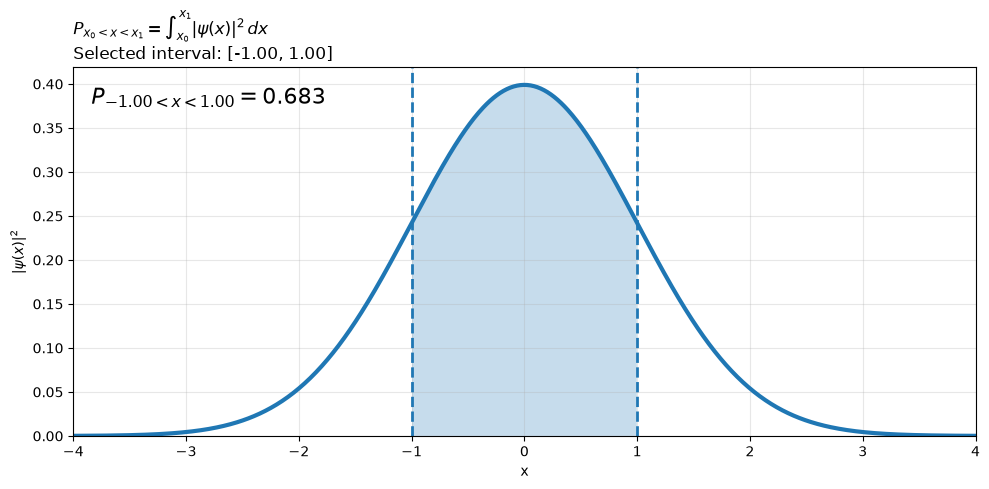

Examples of using probabilistic calculations in QM¶

Example 1: Probability in a region (1D)¶

Take the normalized wavefunction on $[0,1]$: $\psi(x)=\sqrt{3}\,x$. Then $p(x)=|\psi(x)|^2=3x^2$.

• Probability that the particle lies in $[a,b]\subset[0,1]$:

• Concrete numbers, say $[0.3,0.6]$:

Example 2: 3D slice probability (separable state)¶

Let $\psi(x,y,z)=\sqrt{27}\,xyz$ on the unit cube $[0,1]^3$ (this is normalized since $|\psi|^2=27x^2y^2z^2$ and $\int_0^1 x^2dx=\tfrac13$, so $27(\tfrac13)^3=1$).

• Probability the particle is inside the rectangular box $[a_x,b_x]\times[a_y,b_y]\times[a_z,b_z]$:

Example 3: Averages and variance from a PDF¶

For $\psi(x)=\sqrt{3}\,x$ on $[0,1]$ (so $p(x)=3x^2$):

• Mean position:

• Mean square position:

• Variance and standard deviation:

Example 4: Operator expectations (momentum/energy in a box)¶

Operator rules:

• $\hat{p}=-i\hbar\,\dfrac{d}{dx}$,

• $\hat{H}=-\dfrac{\hbar^2}{2m}\dfrac{d^2}{dx^2}+V(x)$.

Use the infinite square well on $[0,1]$ with $V(x)=0$ inside and $\psi_n(x)=\sqrt{2}\sin(n\pi x)$, which is normalized.

• Momentum expectation:

(the integrand is odd over a full sine half-wave, or integrate by parts with vanishing boundary terms).

• Momentum squared:

• Energy (since $\hat{H}=\hat{p}^2/2m$ inside the well):