Diffusion

import numpy as np
import scipy 
import ipywidgets as widgets
import matplotlib.pyplot as plt

%matplotlib inline

Microscopic aspects of Diffusion

• Einstein developed a theory of diffusion based on random walk ideas and obtained a key equation relating mean square displacement of particle in d dimensions to time \((t = n \Delta t)\). Generate N random walks with \(n\) steps all starting from origin \(r_0=0\).

\[R_n = \sum^{n}_{i=0} r_i\]

• Expressing steps in terms of time increments \(n=\frac{t}{\delta t}\) we compute average over N random walkers in \(d=1,2,3\) dimenion.

\[\langle R^2_n\rangle = \sum_i \sum_j \langle r_i r_j \rangle = \sum_i \langle r^2_i \rangle = \sum_i d \cdot \langle \delta x^2_i \rangle = d \cdot n \cdot \delta x^2\]

\[\langle R^2_n\rangle = d \cdot \frac{t}{\delta t} \cdot \delta x^2\]

• Grouping constants together we define the diffusion coefficient which is expressed in terms of microscopic quantities defined in the random walk model!

\[\langle R^2 (t) \rangle = 2d \cdot D \cdot t\]

\[D = \frac{\langle \delta x^2 \rangle}{2\delta t}\]

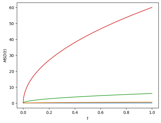
• We end up with a general expression for a mean square displacement as a function of time. Any motion which adheres to this scaling with time will be called diffusive.

\[MSD(t) = 2d D \cdot t^{1/2}\]

d=3 
t= np.linspace(0, 1, 10000)

for D in [0.01, 0.1, 1, 10]:
    
    plt.plot(t, 2*d *D * t**0.5)
    #plt.loglog(t, 2*d *D * t**0.5)

plt.ylabel('$MSD(t)$')
plt.xlabel('$t$')

Text(0.5, 0, '$t$')

Brownian motion

Fig. 4 Animation of brownian motion

• The Brownian motion describes the motion of a particle suspended in a solvent consisting of much smaller moleules. The displacement of particle is generatd by a sum of large number of independent random collisions with solvent molecules. Hence we invoke Central Limit Theorem to approximate displacement at each \(dt\) as a normalally idstributed random variable:

\[x(t+dt)-x(t)=N(0,\sqrt{2D dt})\]

• We assume we have started at position \(\mu=0\), and our variance is given by \(\sigma^2=2Dt\), Where D is the diffusion coefficient, which is related to the parameters of the discrete random walk as shown in the lecture.

\[x(t+dt)=x(t)+\sqrt{2D dt} \cdot N(0,1)\]

• In the last step, we re-wrote Brownian motion equation in a convenient way by shifting the normally distributed random variable by mean and scaling by standard deviation \(N(\mu, \sigma^2) = \mu + \sigma N(0,1)\)

def brown(T, N, dt=1, D=1, d=3):
    
    """
    Creates 3D brownian path given:
    time T 
    N=1 trajecotires
    dt=1 timestep
    D=1 diffusion coeff
    returns np.array with shape (N, T, 3)
    """
    
    n = int(T/dt) # how many points to sample
    
    dR = np.sqrt(2*D*dt) * np.random.randn(N, n, d) # 3D position of brownian particle
    
    R = np.cumsum(dR, axis=1) # accumulated 3D position of brownian particle
    
    return R

R=brown(T=3000, N=1000)
print(R.shape)

(1000, 3000, 3)

def brownian_plot(t=10):
    
    fig, ax = plt.subplots(ncols=2)
    
    ax[0].plot(R[:5, :t, 0].T, R[:5, :t, 1].T);
    
    ax[1].hist(R[:, 10, 0], density=True, color='red')
    ax[1].hist(R[:, t, 0], density=True)
    
    ax[1].set_ylim([0,0.1])
    
    ax[0].set_ylim([-200, 200])
    ax[0].set_xlim([-200, 200])
    
    fig.tight_layout()

import holoviews as hv
hv.extension('plotly')

plots = []
for i in range(10):
    
    plot = hv.Path3D(R[i,:,:], label='3D random walk').opts(width=600, height=600, line_width=5)
    plots.append(plot)
    
hv.Overlay(plots) 

rw_curve = [hv.Curve((R[i,:,0], R[i,:,1])) for i in range(10)]

xdist = hv.Distribution(R[:,10,0], ['X'], ['P(X)'])
ydist = hv.Distribution(R[:,10,1], ['Y'], ['P(Y)'])

hv.Overlay(rw_curve) << ydist << xdist

Diffusion Equation

• The probability distribution of individual random walkers \(\rho({\bf r},t)\) as a function of time \(t\) and displacement from origin \({\bf r}\) follows an diffusion equation which was formulated empirically and known as Fick’s laws. This equation can describe diffusion of large number of random walkers starting from initial condition. For instance dispersion of color die in a solution or diffusion of perfume molecules in the room.

\[\frac{\partial\rho ({\bf r}, t)}{\partial t} = \mathcal{D}\nabla^2\rho({\bf r}, t)\]

• Diffusion equation is a 2nd order PDE! Unlike Netwon’s or Schrodinger equations diffusion equation shows irreversible behavior.The diffusion coefficient \(D\) has of units \([L^2]/[T]\).

• For the case of free diffusion the equation is exactly solvable. But in general reaction-diffusion PDEs difficult to solve analytically. Can solve PDE numerically by writing derivatives as finite differences!

• An important special case solution is free diffusion for 1D case. Notice that it is gaussian with MSD that we derived in CLT and LLN sections \(\sigma(t)=\sqrt{2{D}t}\). You may heck that this is indeed a solution by plugging into the diffusion equation!

\[\rho(x,t) = \frac{1}{\sqrt{2\pi \sigma(t)^2}}\exp\left(-\frac{x^2}{2\sigma(t)^2}\right),\]

def sigma(t, D = 1):
    return np.sqrt(2*D*t)

def gaussian(x, t):
    return  1/np.sqrt(2*np.pi*sigma(t)**2) * np.exp(-x**2/(2*sigma(t)**2)) #

def diffusion(t=1):
    
    R = brown(T=101, N=1000)
    x = np.linspace(-20, 20, 100)
    
    plt.plot(x, gaussian(x, t), label=f'Diff eq solution at t={t}', color='black')
    
    plt.hist(R[:,t,0], density=True, label='brownian diffusion sim', color='green', alpha=0.6)
    
    plt.legend()
    plt.ylabel('$p(x)$')
    plt.xlabel('$x$')
    plt.xlim([-25, 25])
    plt.ylim([0, 0.5])

widgets.interact(diffusion, t=(1, 100))

<function __main__.diffusion(t=1)>