Non-boltzman (enhanced) sampling ideas#
Umbrella Sampling in the 2D Ising Model and Computation of \( F(M) \)#
In the 2D Ising model, the magnetization \( M = \sum_{i,j} s_{i,j} \) serves as a natural order parameter.
However, direct sampling of the full distribution of \( M \) is often inefficient—particularly in systems near criticality or with metastable states—because rare magnetization states are seldom visited in unbiased simulations.
Umbrella sampling is a technique that improves sampling across the full magnetization range by adding a biasing potential that encourages the system to explore specified regions of phase space. Specifically, harmonic umbrella potentials of the form
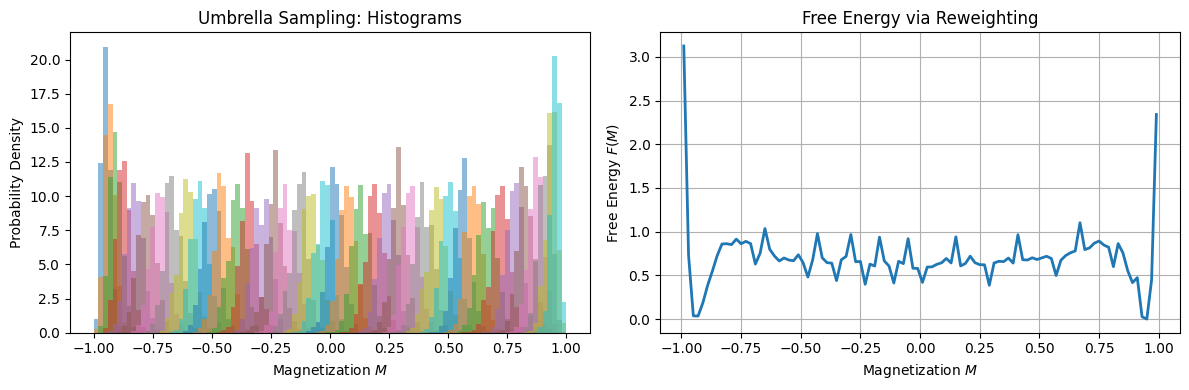
These biased potentails are applied in separate simulations centered at different target magnetizations \( M_0 \). This produces overlapping biased histograms of \( M \).
To recover the unbiased free energy profile \( F(M) \) from these biased distributions, we apply either:
Histogram reweighting: Undo the bias using weights \( \exp(\beta U_{\text{bias}}) \) and stitch histograms together.
MBAR or WHAM: Statistically optimal reweighting of all biased samples to compute \( F(M) = -k_B T \ln P(M) \) with uncertainty estimation.
The resulting \( F(M) \) curve characterizes the thermodynamic landscape of the Ising model and reveals signatures of symmetry breaking, phase transitions, and metastability.
Show code cell source
import matplotlib.pyplot as plt
import numpy as np
from numba import njit

@njit
def compute_total_energy(spins, J, B):
    N = spins.shape[0]
    E = 0.0
    for i in range(N):
        for j in range(N):
            S = spins[i, j]
            neighbors = spins[(i+1)%N, j] + spins[i, (j+1)%N]
            E -= J * S * neighbors
            E -= B * S
    return E

@njit
def run_umbrella_ising2d(N, T, J, B, M0, k_bias, n_steps, out_freq):
    spins = 2 * (np.random.rand(N, N) < 0.5) - 1
    E_t = compute_total_energy(spins, J, B)
    M_t = np.sum(spins)

    n_out = n_steps // out_freq
    E_out = np.empty(n_out)
    M_out = np.empty(n_out)

    k = 0
    for step in range(n_steps):
        i = np.random.randint(N)
        j = np.random.randint(N)
        S = spins[i, j]
        neighbors = spins[(i+1)%N, j] + spins[(i-1)%N, j] + spins[i, (j+1)%N] + spins[i, (j-1)%N]
        dE = 2 * S * (J * neighbors + B)

        M_new = M_t - 2 * S
        dU = 0.5 * k_bias * (M_new - M0)**2 - 0.5 * k_bias * (M_t - M0)**2
        d_total = dE + dU

        if d_total <= 0 or np.random.rand() < np.exp(-d_total / T):
            spins[i, j] = -S
            E_t += dE
            M_t = M_new

        if step % out_freq == 0:
            E_out[k] = E_t / N**2
            M_out[k] = M_t / N**2
            k += 1

    return E_out, M_out
N = 20
T = 2.0
J = 1.0
B = 0.0
n_steps = 1000000
out_freq = 100
k_bias = 0.01

M0_values = np.linspace(-1.0, 1.0, 40)
all_mags = []

for M0 in M0_values:
    _, M_out = run_umbrella_ising2d(N, T, J, B, M0*N**2, k_bias, n_steps, out_freq)
    all_mags.append(M_out)
Basic Reweighting#
import numpy as np
import matplotlib.pyplot as plt

# === Parameters and binning ===
beta=1/T
nbins = 100
bin_edges = np.linspace(-1, 1, nbins + 1)
bin_centers = 0.5 * (bin_edges[1:] + bin_edges[:-1])
P_unbiased = np.zeros(nbins)

# === Set up figure with 1 row, 2 columns ===
fig, ax = plt.subplots(1, 2, figsize=(12, 4))

# === Plot overlapping histograms ===
for mags in all_mags:
    ax[0].hist(mags, bins=bin_edges, density=True, alpha=0.5)
ax[0].set_xlabel("Magnetization $M$")
ax[0].set_ylabel("Probability Density")
ax[0].set_title("Umbrella Sampling: Histograms")

# === Reweight and compute unbiased distribution ===
for M0, mags in zip(M0_values, all_mags):

    U = 0.5 * k_bias * N**4 * (mags - M0)**2
    hist, _ = np.histogram(mags,
                           bins=bin_edges,
                           weights=np.exp(-beta * U))
    P_unbiased += hist

# Normalize the unbiased probability density
P_unbiased /= np.sum(P_unbiased * np.diff(bin_edges))

# Compute free energy: F(M) = -kT ln P(M)
F_reweighted = -np.log(P_unbiased + 1e-12)
F_reweighted -= np.nanmin(F_reweighted)

# === Plot F(M) ===
ax[1].plot(bin_centers, F_reweighted, lw=2)
ax[1].set_xlabel("Magnetization $M$")
ax[1].set_ylabel("Free Energy $F(M)$")
ax[1].set_title("Free Energy via Reweighting")
ax[1].grid(True)

plt.tight_layout()
plt.show()
Reweighting using pymbar#
!pip install pymbar
Collecting pymbar
  Downloading pymbar-4.0.3-py3-none-any.whl.metadata (1.2 kB)
Requirement already satisfied: numpy>=1.12 in /opt/hostedtoolcache/Python/3.8.18/x64/lib/python3.8/site-packages (from pymbar) (1.24.4)
Requirement already satisfied: scipy in /opt/hostedtoolcache/Python/3.8.18/x64/lib/python3.8/site-packages (from pymbar) (1.10.1)
Collecting numexpr (from pymbar)
  Downloading numexpr-2.8.6-cp38-cp38-manylinux_2_17_x86_64.manylinux2014_x86_64.whl.metadata (8.0 kB)
Downloading pymbar-4.0.3-py3-none-any.whl (107 kB)
Downloading numexpr-2.8.6-cp38-cp38-manylinux_2_17_x86_64.manylinux2014_x86_64.whl (384 kB)
Installing collected packages: numexpr, pymbar
Successfully installed numexpr-2.8.6 pymbar-4.0.3
Show code cell source
import numpy as np
import matplotlib.pyplot as plt
from pymbar import FES

# === USER INPUTS ===

beta = 1.0 / T
k_bias = 0.01
M0_values = np.linspace(-1, 1, 20)  # umbrella centers

# === COLLECT ALL MAGNETIZATION DATA ===
M_all = np.concatenate(all_mags)
N_total = len(M_all)
N_k = np.array([len(m) for m in all_mags])
N_windows = len(M0_values)

# === BUILD REDUCED POTENTIAL MATRIX u_kn ===
u_kn = np.zeros((N_windows, N_total))
start = 0
for k, (M0, Nk) in enumerate(zip(M0_values, N_k)):
    M_window = M_all[start:start+Nk]
    u_kn[k, start:start+Nk] = beta * 0.5 * k_bias * (M_window * N**2 - M0)**2
    start += Nk

# === FES INPUTS ===
fes = FES(u_kn, N_k)
u_n = u_kn[0, :]
x_n = M_all.reshape(-1, 1)

# === DEFINE UNEQUALLY POPULATED BINS ===
nbins = 100
x_sorted = np.sort(M_all)
bin_edges = np.append(x_sorted[::N_total//nbins], x_sorted.max() + 0.01)
bin_centers = 0.5 * (bin_edges[1:] + bin_edges[:-1])
histogram_parameters = {'bin_edges': [bin_edges]}

# === GENERATE FES ===
fes.generate_fes(u_n=u_n, x_n=x_n,
                 fes_type='histogram',
                 histogram_parameters=histogram_parameters)

# === QUERY FES AT DATA POINTS (like pymbar docs) ===
results = fes.get_fes(x_n, uncertainty_method='analytical')
f_i = results['f_i']
df_i = results['df_i']

# === BIN THE FREE ENERGY BACK INTO BIN_CENTERS ===
indices = np.digitize(M_all, bin_edges) - 1
F_binned = np.zeros(len(bin_centers))
dF_binned = np.zeros(len(bin_centers))
counts = np.zeros(len(bin_centers))

for i, idx in enumerate(indices):
    if 0 <= idx < len(bin_centers):
        F_binned[idx] += f_i[i]
        dF_binned[idx] += df_i[i]**2
        counts[idx] += 1

mask = counts > 0
F_binned[mask] /= counts[mask]
dF_binned[mask] = np.sqrt(dF_binned[mask]) / counts[mask]

# Normalize
F_binned -= np.nanmin(F_binned[mask])

# === PLOT ===
plt.errorbar(bin_centers[mask], F_binned[mask], yerr=dF_binned[mask], fmt='o-', capsize=2)
plt.xlabel("Magnetization $M$")
plt.ylabel("Free Energy $F(M)$")
plt.title("Free Energy Profile from Umbrella Sampling (pymbar FES)")
plt.grid(True)
plt.tight_layout()
plt.show()
Warning on use of the timeseries module: If the inherent timescales of the system are long compared to those being analyzed, this statistical inefficiency may be an underestimate. The estimate presumes the use of many statistically independent samples. Tests should be performed to assess whether this condition is satisfied. Be cautious in the interpretation of the data.
********* JAX NOT FOUND *********
 PyMBAR can run faster with JAX
 But will work fine without it
Either install with pip or conda:
      pip install pybar[jax]
               OR
      conda install pymbar
*********************************
---------------------------------------------------------------------------
IndexError                                Traceback (most recent call last)
Cell In[5], line 26
     23     start += Nk
     25 # === FES INPUTS ===
---> 26 fes = FES(u_kn, N_k)
     27 u_n = u_kn[0, :]
     28 x_n = M_all.reshape(-1, 1)

File /opt/hostedtoolcache/Python/3.8.18/x64/lib/python3.8/site-packages/pymbar/fes.py:165, in FES.__init__(self, u_kn, N_k, verbose, mbar_options, timings, **kwargs)
    162     self.timings = True
    164 if mbar_options == None:
--> 165     fes_mbar = pymbar.MBAR(u_kn, N_k)
    166 else:
    167     # if the dictionary does not define the option, add it in
    168     required_mbar_options = (
    169         "maximum_iterations",
    170         "relative_tolerance",
   (...)
    175         "x_kindices",
    176     )

File /opt/hostedtoolcache/Python/3.8.18/x64/lib/python3.8/site-packages/pymbar/mbar.py:410, in MBAR.__init__(self, u_kn, N_k, maximum_iterations, relative_tolerance, verbose, initial_f_k, solver_protocol, initialize, x_kindices, n_bootstraps, bootstrap_solver_protocol, rseed)
    407 else:
    408     np.random.seed(rseed)
--> 410 self.f_k = mbar_solvers.solve_mbar_for_all_states(
    411     self.u_kn, self.N_k, self.f_k, self.states_with_samples, solver_protocol
    412 )
    414 if n_bootstraps > 0:
    415     self.n_bootstraps = n_bootstraps

File /opt/hostedtoolcache/Python/3.8.18/x64/lib/python3.8/site-packages/pymbar/mbar_solvers.py:993, in solve_mbar_for_all_states(u_kn, N_k, f_k, states_with_samples, solver_protocol)
    990     f_k_nonzero = np.array([0.0])
    991 else:
    992     f_k_nonzero, all_results = solve_mbar(
--> 993         u_kn[states_with_samples],
    994         N_k[states_with_samples],
    995         f_k[states_with_samples],
    996         solver_protocol=solver_protocol,
    997     )
    999 f_k[states_with_samples] = np.array(f_k_nonzero)
   1001 # Update all free energies because those from states with zero samples are not correctly computed by solvers.

IndexError: index 20 is out of bounds for axis 0 with size 20
Simulated annealing#
Is a widely used Monte Carlo technique used for numerical optimization In chemical and biological applications simulated annealing is used for finding global minima of a complex multidimensional energy functions>
Original paper: S. Kirkpatrick, C. D. Gelatt, Jr., M. P. Vecchi, Science 220, 671-680 (1983)
Simulated annealing in a nutshell#
Introduce (artificial) temperature parameter \(T\)
Sample with metropolis algorithm where the acceptance probability takes the form \(min (1, e^{-\Delta f/T})\)
Here \(f\) can be any function we want to minimize (not only energy)
For finding maximum simply change the sign: \(min (1, e^{+\Delta f/T})\)
Slowly reduce the temperature
“Slow cooling” is the main idea of simulated annealing
#
very high \(T\) |
very low \(T\) |
|---|---|
almost all updates are accepted |
only updates that decrease the energy are accepted |
random configurations/explore entire space |
descend towards minimum |
high energy |
low energy but might get stuck in local minimum |
if we slowly cool from high \(T\) to low \(T\) we will explore the entire space until we converge to the (hopefully) global minimum
success is not guaranteed, but the methods works very well with good cooling schemes
Inspiration: annealing in metallurgy.
This is a great method to tackle NP-hard optimization problems, such as the traveling salesman!
Cooling schedules#
slow cooling is essential: otherwise the system will “freeze” into a local minimum
but too slow cooling is inefficient…
initial temperature should be high enough so that the system is essentially random and equilibrates quickly
final temperature should be small enough so that we are essentially in the ground state (system no longer changes)
exponential cooling schedule is commonly used
\[\boxed{T(t)=T_0e^{-t/\tau}}\]where \(t\) is the Monte Carlo time and the constant \(\tau\) needs to be determined (usually empirically)
alternative cooling schedules:
linear: \(T(t)=T_0 - t/\tau\) (also widely used)
logarithmic: \(T(t) = c/\log(1+t/\tau)\)
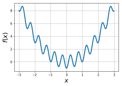
Example: find global minimum of the function via simulated annealing: \(f(x) = x^2 -\cos (4\pi x)\)#
f = lambda x: x*x - np.cos(4*np.pi*x)
xvals = np.arange(-3,3,0.01)

plt.plot(xvals, f(xvals),lw=3)

plt.xlabel("$x$",fontsize=20)
plt.ylabel("$f(x)$",fontsize=20)
plt.grid(True)
Search for global minima of \(f(x)\) using simulated annealing#
def MCupdate(T, x, mean, sigma):

    '''Making a new move by incremening a normal distributed step
    We are exploring function diffusivefly, e.g doing random walk!
    T: temp
    mean, sigma: parameters of random walk
    '''

    xnew = x + normal(mean, sigma)

    delta_f = f(xnew) - f(x)


    if delta_f < 0 or np.exp(-delta_f/T) > rand():

        x = xnew

    return x


def cool(T, cool_t):

    '''Function for educing T after every MC step.

    cool_t: cooling time tau for exponential schedule
    Alternatively we could reduce every N steps.'''

    return T*np.exp(-1/cool_t)
def sim_anneal(T=10, T_min=1e-4, cool_t=1e4, x=2, mean=0, sigma=1):

    '''Simulated annealing search for min of function:

    T=T0:        starting temperature
    T_min:       minimal temp reaching which sim should stop
    cool_t:      colling pace/time
    x=x0:        starting position
    mean, sigma: parameters for diffusive exploration of x'''

    xlog   = []

    while T > T_min:

        x = MCupdate(T, x, mean, sigma)

        T = cool(T, cool_t)

        xlog.append(x)

    return xlog
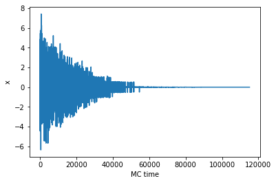
xlog = sim_anneal()

plt.plot(xlog)

plt.xlabel('MC time')
plt.ylabel('x')
print('Final search result for the global minimum: ', xlog[-1])
Final search result for the global minimum: 0.0012962682770579035
@widgets.interact(t_sim=(1,1000))
def viz_anneal(t_sim=1):

    T           = 4
    x           = 2
    cool_t      = 1e4
    mean, sigma = 0, 1

    plt.plot(xvals, f(xvals),lw=3, color='green')

    for t in range(t_sim):

        x = MCupdate(T, x, mean=0, sigma=1)

        T = cool(T, cool_t)

    plt.plot(x, f(x),'o',color='red',ms=20,alpha=0.5)
    plt.ylim(-1,8)
    plt.xlim(-3,3)
    plt.grid(True)
    plt.xlabel('$x$',fontsize=20)
    plt.ylabel('$f(x)$',fontsize=20)
Challanges#
always slightly above true minimum if \(T>0\)
best combined with a steepest descent method
Simulated annealing applied to MCMC sampling of 2D Ising model#
temperature = 10.0    # initial temperature
tempmin = 1e-4        # minimal temperature (stop annealing when this is reached)
cooltime = 1e4        # cooling time tau for exponential schedule

# how long it will take to cool to minimal temperature in MC steps
MCtime = -cooltime*np.log(tempmin/temperature)

# after every MC step we reduce the temperature
def cool(temperature):

    return temperature*np.exp(-1/cooltime)
Parallel tempering#
Simulated annealing is not guaranteed to find the global extremum
Unless you cool infinitely slowly.
Usually need to repeat search multiple times using independent simulations.
Parallel tempering (aka Replica Exchange MCMC)
Simulate several copies of the system in parallel
Each copy is at a different constant temperature \(T\)
Usual Metropolis updates for each copy
Every certain number of steps attempt to exchange copies at neighboring temperatures
Exchange acceptance probability is min(1, \(e^{-\Delta f\Delta\beta}\))
If temperature difference small enough, the energy histograms of the copies will overlap and exhcanges will happen often.
Advantages of replica exchange:
Exchanges allow to explore different extrema
More successful for complex functions/energy landscapes. Random walk in temperature space!
Detailed balance is maintained! (regular simulated annealing breaks detailed balance)
How to choose Temperature distributions for replica exchange MCMC#
A dense temperature grid increases the exchange acceptance rates
But dense T grid takes longer to simulate and more steps are needed to move from one temperature to another
There are many options, often trial and error is needed
exchange acceptance probability should be between about 20% and 80%
exchange acceptance probability should be approximately temperature-independent
commonly used: geometric progression for \(N\) temperatures \(T_n\) between and including \(T_{\rm min}\) and \(T_{\rm max}\) (ensures more steps around \(T_{\rm min}\))
\[T_n = T_{\rm min}\left(\frac{T_{\rm max}}{T_{\rm min}}\right)^{\frac{n-1}{N-1}}\]
make sure to spend enough time before swapping to achieve equilibrium!
parallel tempering simulation#
######## Ising 2D+PT ###########

@njit
def mcmc(spins, J, B, T, n_steps = 10000, out_freq = 1000):

    '''mcmc takes spin configuration and samples with given N,J,B,T
    for n_steps outputing results every out_freq'''

    confs = []
    N = len(spins)

    for step in range(n_steps):

        #Pick random spin
        i, j = randint(N), randint(N)

        #Compute energy change
        z  = spins[(i+1)%N, j] + spins[(i-1)%N, j] + spins[i, (j+1)%N] + spins[i, (j-1)%N]
        dE = 2*spins[i,j]*(J*z + B)

        #Metropolis condition
        if np.exp(-dE/T) > rand():

            spins[i,j] *= -1

        #Store the spin configuration
        if step % out_freq == 0:

            confs.append(spins.copy())

    return confs

@njit
def getE(spins, J, B):

    N = len(spins)
    E = 0

    for i in range(N):
        for j in range(N):

            z = spins[(i+1)%N, j] + spins[(i-1)%N, j] +spins[i,(j+1)%N] +  spins[i,(j-1)%N]

            E += -J*z*spins[i,j]/4 # Since we overcounted interactions 4 times divide by 4.

    return E - B*np.sum(spins) #Field contribution added

@jit
def temper(configs, T):
    '''Randomly pick two adjacent replicas and attempt an exchange'''

    i       = np.random.randint(len(T)-1)
    j       = i+1

    deltaBeta      = 1/T[i] - 1/T[j]

    deltaEnergy    = getE(configs[i][-1], J, B) - getE(configs[j][-1], J, B)

    if np.exp(-deltaBeta*deltaEnergy) > rand():

        #T[i], T[j] = T[j], T[i]
        configs[i][-1], configs[j][-1] = configs[j][-1], configs[i][-1]

    return configs

@jit
def pt_mcmc(N, J, B, T=[1, 0.1], n_exch=1000):

    configs    = [[choice([-1,1], (N,N))] for _ in T]

    # Exchange attemps
    for swap_attempt in range(n_exch):

        configs  = temper(configs, T)

        #mcmc in between exchange attemp
        for i in range(len(T)):

            configs_new = mcmc(configs[i][-1],  J, B, T[i])

            configs[i].extend(configs_new)

    return configs
%%capture

N = 20       # size of lattice in each direction
J = 1        # interaction parameter
B = 0        # magnetic field

T = [5.0, 0.01, 0.0008, 0.0007, 0.00016, 0.00010]

n_exch   = 1000
n_steps  = 10000
out_freq = 100

configs = pt_mcmc(N, J, B, T, n_exch)
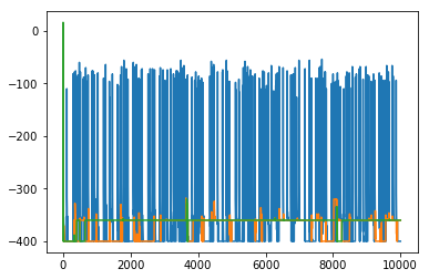
E1 = [getE(spins, J,B) for spins in configs[1]]
E2 = [getE(spins, J,B) for spins in configs[2]]
E3 = [getE(spins, J,B) for spins in configs[3]]
plt.plot(E1)
plt.plot(E2)
plt.plot(E3)
[<matplotlib.lines.Line2D at 0x7fc0d94e2590>]
@widgets.interact(i=(0,999))
def plot_image(i=1):

    fig,ax = plt.subplots(figsize=(8,8))
    ax.imshow(configs[0][i])
Problems#
Umbrella Sampliing
Use umbrealla sampling to obtain free energy profile as a function of magnetization below \(T_c\) at \(T_c\) and above \(T_c\). E.g \(T=2, 2.5, 3\) Consider using the inputs from adjecent umbrella simulations. E.g input for umbrella 4 can come from umbrella 3 to speed up simulations.
Simulated Annealing
Complete the simulated annealing part of the code for finding minimum energy in Ising models. Test your code with field on and off.
Parallel Tempering
Use parallell tempering to enhance the sampling at \(T =1\) by coupling 8 replicas with \(T>1\). Find the optimal T spacing between replicas, Calculate histograms of magnetization to show enhancement of sampling with respect to constant T MCMC.