Open Systems#
Fig. 21 Open systems are characterized by variable number of particles and energy#
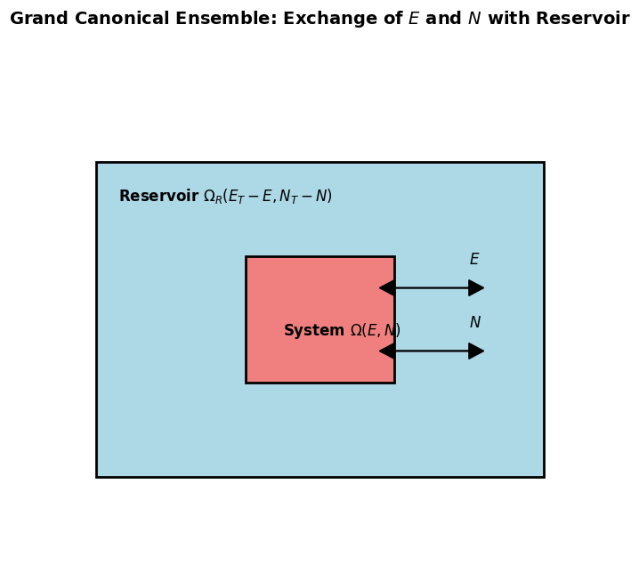
Grand Canonical Ensemble#
Consider small system \( S \) in thermal and particle exchange with a large reservoir \( R \).
The total system \( S + R \) is isolated: total energy \( E_{\text{tot}} = E + E_R \), total particle number \( N_{\text{tot}} = N + N_R \).
Total volume is constant, and the reservoir is much larger: \( E \ll E_R \), \( N \ll N_R \).
Microstate Probability#
The probability that the system has energy \( E \) and particle number \( N \) is proportional to the number of microstates of the reservoir with \( E_R = E_{\text{tot}} - E \), \( N_R = N_{\text{tot}} - N \):
Define entropy of the reservoir \( S_R = k_B \ln \Omega_R \). Then:
Expand to first order:
Use thermodynamic definitions:
Grand Canonical Distribution and Partition Function#
Define the grand canonical partition function:
where:
\( z = e^{\beta \mu} \) is called the fugacity.
\( Z_N = \sum_{\text{states at fixed } N} e^{-\beta E} \) is the canonical partition function at fixed \( N \)
The microstate probability in grand canonical ensemble is:
The macrostate probability over different energy values in grand canonical ensemble is:
Grand-Canonical distribution
Connections with \(NVE\) and \(NVT\)#
Statistical Dominance of Average Energy and Particle Number#
Recall that the canonical ensemble emerges by weighting microcanonical contributions at different energies with an exponential factor \( e^{-\beta E} \).
Similarly, the grand canonical ensemble arises by further summing over all particle numbers \( N \), each weighted by the fugacity factor \( e^{\beta \mu N} \). This yields the grand canonical partition function:
\[ \Xi(T, V, \mu) = \sum_{N=0}^{\infty} \left[ \sum_i e^{-\beta E_i} \right] e^{\beta \mu N} = \sum_{N=0}^{\infty} Z(N, V, T) \, e^{\beta \mu N} \]In the thermodynamic limit, the sum is dominated by the most probable energy and particle number, giving:
\[ \Xi \approx e^{-\beta (F - \mu \bar{N})} = e^{-\beta (\bar{E} - T S - \mu \bar{N})} = e^{-\beta \Psi(T, V, \mu)} \]We identify a new thermodynamic potential for the grand canonical ensemble that plays same role as free energy in canonical ensemble:
Grand potential
Thermodynamics and Legendre transform#
In thermodynamics grand potential \( \Psi \) is derived from the internal energy \( E(S, V, N) \) via a Legendre transform that replaces the natural variables \( S \to T \) and \( N \to \mu \):
\[ E(S, V, N) \rightarrow E - \left( \frac{\partial E}{\partial S} \right) S - \left( \frac{\partial E}{\partial N} \right) N = E - T S - \mu N \]
Grand Potential and Pressure#
Using Euler’s relation for extensive thermodynamic variables:
\[ E = T S + P V + \mu N \]Substituting into the definition of \( \Psi \), we find:
\[ \Psi = E - T S - \mu N = -P V \]Hence, the grand potential is directly related to the pressure and volume:
\[ {\Psi(T, V, \mu) = -P V} \]
Fluctuations in particle numbers#
We once again find that in case of fluctuating quantities (energy in NVT) the relative fluctuation scales as \(N^{-1/2}\) a hallmark of Central Limit Theorem!
Using thermodynamics we could also link number fluctuations with isothermal compressibility \(\kappa_T\)
The relationship is analogus to what we had established in \(NVT\) between energy flcutuations and heat capcity.
It takes a bit more work manipulating variables to get there in this case. See belwo for derivation:
Ideal Gas in the Grand Canonical Ensemble#
We begin by considering an ideal gas of indistinguishable, non-interacting particles in a volume \( V \), in thermal and chemical equilibrium with a reservoir at temperature \( T \) and chemical potential \( \mu \).
The canonical partition function for \( N \) particles is:
Where the thermal de Broglie wavelength is:
Grand Canonical Partition Function#
To account for fluctuations in particle number, we compute the grand canonical partition function:
Fugacity: \( z = e^{\beta \mu} \), a dimensionless measure of how favorable it is to add a particle to the system.
The average particle number is then obtained by taking first derivative withr espect to N
Chemical Potential in Terms of Pressure and Density#
We can invert the relation for \( \langle N \rangle \) to express the chemical potential:
Noting that for an ideal gas \( p = \frac{N k_B T}{V} \), this becomes:
Chemical Potential of Ideal Gas
\( \mu^0(T)\) is the reference chemical potential at unit pressure.
Number Fluctuations#
In the grand canonical ensemble, number fluctuations are given by:
So the standard deviation \( \sigma_N \sim \sqrt{N} \), and relative fluctuations vanish as \( N^{-1/2} \) in the thermodynamic limit.
Isothermal Compressibility#
We relate number fluctuations to the isothermal compressibility \( \kappa_T \):
This is the well-known result for the ideal gas compressibility:
\( \kappa_T = \frac{1}{p} \geq 0 \), a positive quantity ensuring mechanical stability.
Molecular Adsorption of Ideal Gas on Surfaces#
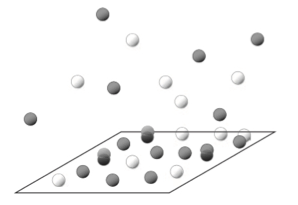
One Site–One Molecule Model#
We consider a simple model where each adsorption site can hold at most one molecule. The surface is in thermal and chemical equilibrium with a gas reservoir at temperature \( T \) and chemical potential \( \mu \).
Each site has two possible states:
Empty: energy \( E = 0 \)
Occupied: energy \( E = \epsilon \)
Then the grand partition function for a single site is:
\( N \) Independent Sites#
If there are \( N \) independent and identical adsorption sites, then the total grand partition function is:
Since the sites do not interact, their contributions multiply.
Average Number of Adsorbed Molecules#
The average occupation number per site is:
The total number of adsorbed molecules is:
Average Energy#
The average energy per site is:
The total energy of the system is:
Connecting to Pressure#
For an ideal gas in the reservoir, the chemical potential is related to pressure via:
Substituting this into the expression for \( \langle n \rangle \):
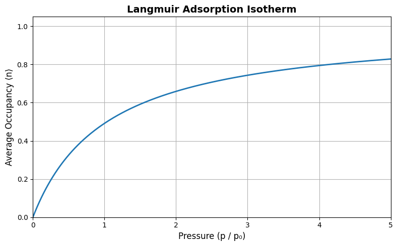
and thus the total number of adsorbed molecules becomes:
This is the Langmuir adsorption isotherm, describing how the fraction of occupied adsorption sites depends on gas pressure. It captures saturation behavior as \( p \to \infty \), where \( \langle n \rangle \to 1 \).
Show code cell source
import matplotlib.pyplot as plt
import numpy as np

# Parameters
T = 298  # Temperature in K
epsilon = 10 * 1.38e-23  # Adsorption energy in J (10 k_B T)
k_B = 1.38e-23  # Boltzmann constant
beta = 1 / (k_B * T)
p0 = 1  # Reference pressure (arbitrary units)

# Pressure range
p = np.linspace(0, 5, 500)

# Langmuir isotherm
n_avg = p / (p0 * np.exp(beta * epsilon) + p)

# Plotting
plt.figure(figsize=(8, 5))
plt.plot(p, n_avg, lw=2)
plt.xlabel('Pressure (p / p₀)', fontsize=12)
plt.ylabel('Average Occupancy ⟨n⟩', fontsize=12)
plt.title('Langmuir Adsorption Isotherm', fontsize=14, weight='bold')
plt.grid(True)
plt.ylim(0, 1.05)
plt.xlim(0, 5)
plt.tight_layout()
plt.show()
Exercise: Multi-stide binding of molecular gas with internal states
Write down partition function for these scenarious
Molecule A binds to one site and adopts 2 conformations.
Two molecules of B can bind one site. When one molecle is bound it has one conformation and when two bound there are 5 conformations.
Chemical Equilibrium in gas mixtures#
For each species \( i \), the canonical partition function is:
where:
\( \lambda_i = \frac{h}{\sqrt{2\pi m_i k_B T}} \) is the thermal wavelength,
\( q_i^{\text{int}} \) is the internal partition function (rotations, vibrations, etc.),
\( N_i \) is the number of molecules of species \( i \).
For conenvience lets use the Helmholtz free energy (same result with Gibbs Free energy):
Using Stirling’s approximation \( \log N_i! \approx N_i \log N_i - N_i \):
Equilibrium via minimization of free energy#
Now, we consider a chemical reaction:
We introduce an extent of reaction \( \xi \) which measures how far reaction has progressed from reactants to products:
We minimize \( F(\xi) \) at constant \( T, V \) by setting:
Computing the derivative:
with \( \nu_i \) the stoichiometric coefficient (\( < 0 \) for reactants, \( > 0 \) for products). Or we can write it in terms of positive stochimoetric coefficients:
Chemical potential and Chemical equilibrium
So the equilibrium condition is:
Exponentiating both sides we relate ration of equilibrium numbers or concentrations to partition functions
Equilibrium Constant from Partition Functions
Problems#
\(NVT-NVE-\mu V T\)#
Consider a three level single particle system with five microstates with energies 0, ε, ε, ε, and 2ε. What is \(\Omega(\epsilon n)\) n=0,1,2 for this system? What is the mean energy of the system if is in equilibrium with a heat bath at temperature T ?
Derive an expression for the chemical potential of an ideal gas using clssical mechanics model for energy \(E=\frac{p^2}{2m}\) in the \(\mu VT\) ensemble evaluate the fluctuations in particle number.
Consider a system in equilibrium with a heat bath at temperature \(T\) and a particle reservoir at chemical potential \(\mu\). The system can have a minimum of one and a maximum of four distinguishable particles. The particles in the system do not interact and can be in one of two states with energies zero or \(\Delta\). Determine the (grand) partition function of the system.
Combine the Gibbs formula of Entropy \(S=-k_B \sum_i p_i log p_i\) with the Grand canonical prbability distribution \(P(E_i,N)=\frac{e^{-\beta E_i+ \beta \mu N}}{Z_G}\) to show that \(\beta PV=log Z_G\)
Derive partition function for a pressure ensemble \((T, p, N)\) and show its connection with microcanonical ensemble \(N V E\)
At a given temperature T a surface with \(N_0\) adsorption centers has on average \(N\neq N_0\) number of adsorbed molecules. Suppose hat there are no interactions between molecules.
Show that the chemical potential of adsorbed gas is given by: \(\mu = k_B T log \frac{N}{N_0 - N a(T)}\)
What is the meaning of \(a(T)\)