Photons and Phonons#
Lattice vibrations and phonon gas#
![]()
\(\omega(k)\) defines dispersion relation
\(v_g = \frac{d\omega(k)}{dk}\) group velocity of traveling waves in the material.
In 1D there are discrete number of wavelengths that are possible; \(2L, 2L/2, ...2L/n\) and hence \( 2\pi n/L\) which follows from imposing periodic boundary conditions \(cos kaN=1\)
Low frequency regime \(ka \ll 1\) we have \(\omega \approx (Ca ^2/m)^{1/2} k\) simple dispersion relation.
Quantization of harmonic degrees of freedom#
Conisder a model of a solid with atoms repreented as \(N\) localized and noninteracting quantim 1D oscillators with frequencies \(\omega_i\). The solid is in thermal contact with a heat bath at temperature \(T\).
The energy of this solid will be a sum of oscillator energies defined in terms of quantum numbers \(n_1, n_2, ... n_N\)
Partition function can be decouples intp product of exponentials corresponding to disting mode frequencies \(\omega_i\)
We recongnize the last factor as grand canonical partition function \(Y(\beta, 0)\) for bosons with \(\mu=0\). This is a nice mathematical observation allowing us to describe photons and phonons via grand canonical partion function by setting chemical potential to zero.
Average occupancy of an oscillator
Total energy
Debye Theory of solidsm#
Debye makes a continuous approximation of frequencies to express total energy of a solid as an integral over a finite range of frequencies. The physical basis of this approximation is treating lattice vibration as long-wavelength waves \(\lambda\gg a\) propagating in the crystal by disregarding short wavelength oscillations.
Waves propagate in non-dispersive medium hence \(\omega(k)=vk\) dipendence takes a simple form with group velocity coinciding with sound velocity \(v_g= \frac{d\omega}{dk}=v\).
Accounting for transverse and longitudinal waves we mulitply the expression by three and replace velocity by average velocity: \(\frac{3}{\bar{v}^3} =\frac{1}{v_T^3}+ \frac{2}{v_L^3} \)
The equation is based on large wavelength approximation (low frequency). This is why the cutoff in frequency range is introduced called Debye frequency, \(\omega_D\). To renormalize the frequencies such that the total number of them is 3N
Integration allows to replace average velocity with Debye cutoff frequency: \(\omega^3_D = 6\pi^2 \frac{N}{V}\bar{v}^3\)
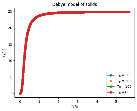
Heat capacity of Debye solid accurately captures low temperature regime#
We now write down heat capacity \(C_v(T)=\frac{dE}{dT}\) expressed in terms of variables
\(x =\frac{\hbar \omega}{k_BT}\)
\(x_D = \frac{\hbar \omega_D}{k_BT}=\frac{\Theta_D}{T}\)
import numpy as np
import scipy
from scipy.integrate import quad
from scipy.constants import k , N_A, hbar

import matplotlib.pyplot as plt

def debye (T, T_D=105, N=6e23) :
    '''Returns the exact heat capacity of Debye model given the number of modes debye     temperature constant and temperature'''

    def f(x):
        return  x**4 * np.exp(x)/(np.exp(x)-1)**2


    C = np.zeros(len(T))

    for i, t in enumerate(T):

        C[i] = ( 9*N*k*(t/T_D)**3 ) * quad(f, 0 , T_D/t)[0]

    return C
Ts = np.linspace(1, 500, 1000)

for T_D in [380, 200, 105, 88]:

    plt.plot(Ts/T_D, debye(Ts, T_D=T_D), '-o', label=f'$T_D = {T_D}$')

plt.xlabel('$T/T_D$')
plt.ylabel('$C_v(T)$')
plt.legend()
plt.title('Debye model of solids')
/tmp/ipykernel_2195/200287254.py:12: RuntimeWarning: overflow encountered in scalar power
  return  x**4 * np.exp(x)/(np.exp(x)-1)**2
Text(0.5, 1.0, 'Debye model of solids')
The photon gas#
Photon statistics is obtained by making use of Bose-Einstein distribution by setting \(\mu=0\):
In the non-dispersive media we have \(\omega =c k\).
Using De-brolgie relation \(p=\hbar k=\hbar\omega/c\) we express density of states as a function of \(\omega\) and multiply the expression by two to acount for two perpendicular polarization states of electromagnetic waves
The mean number of photons
The total radiation energy per volume
Radiation as a function of wavelength \(\lambda = 2\pi c/\omega\):
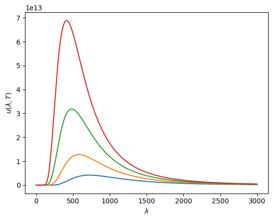
Planck’s law of blacbody radiation#
Planck law explains why spectrum shifts towards blue as temperature increases
The total energy density \(u(T) = E/V\) of a radiation field at temperature T is finite and there is no ultraviolet catastrophe which was predicted by classical reasning prior to QM.
Since we know \(C_v\sim T^3\) temeprature dependence of phons this should be expected. Thus we realize that mathematically low temperature heat of crystals and radiation field problem are the same!
In the classical limit \(\hbar\rightarrow 0\) we get:
This is a Raleigh-Jeans formula dervied using classical physics. Upon integration it diverges giving ultraviolet catstrophe. The divergence is due to high frequency modes.
In the high frequency limit \(\hbar\omega \gg k_B T\) Planck’s law goes to:
from scipy.constants import c, k, h


def planck(wav, T):

    return 2.0*h*c**2 / ( (wav**5) * (np.exp(h*c/(wav*k*T)) - 1.0) )


wavs = np.arange(1e-9, 3e-6, 1e-9) # nanometer units

for Ts in [4000, 5000, 6000, 7000 ]:

    plt.plot(wavs*1e9,  planck(wavs, Ts))

plt.xlabel('$\lambda$')
plt.ylabel('$u(\lambda, T)$')
/tmp/ipykernel_2195/1557676303.py:6: RuntimeWarning: overflow encountered in exp
  return 2.0*h*c**2 / ( (wav**5) * (np.exp(h*c/(wav*k*T)) - 1.0) )
Text(0, 0.5, '$u(\\lambda, T)$')
Problems#
Problem 1: Bose-Einstein and Fermi-diract distributions#
Compute particle occupation number fluctuations for non-interacting fermions and bosons.
For the classical gas, the number distribution in a small volume obey the Poisson distribution. Using the fluctuations computed in (1) show that in the low density regime quantum and classical gases display Poisson distribution of numbers. (Hint: Recall that for Poisson distribution \(\mu=\sigma^2\))
Consider a fermion gas. Plot occupation number \(\langle n_i \rangle\) of energy level \(\epsilon_i\) as a function of \(\epsilon_i/k_{BT}\) for several values of chemical potential \(\mu=-k_{B}T,5k_{B}T,10k_{B}T\). Comment on the trend.
While keeping the \(\mu=10k_{B}T\) make plots with different temperatures and comment on the trend.
Set \(\mu=0\) for simplicity and on the same graph plot probability distribution for Fermi-Dirac, Bose-Einstein and Boltzmann statistics.
Problem 2: Einstein and Debye model of solids#
What are the normal modes and how they help with computing partiion functions of solids.
Explain what aspect of Einstein and Debye models makes for a better agreement with heat capacity of solids at low temperatures.
Explain the discrepancy in temeprature dependence between Einstein and Debye models \(C_v(T)\). What aspect makes Debye model capture low temperature limit.
Explain in few short sentences what is the take home message of this paper https://www.researchgate.net/publication/6046921_Specific_Heat_and_Thermal_Conductivity_of_Solid_Fullerenes