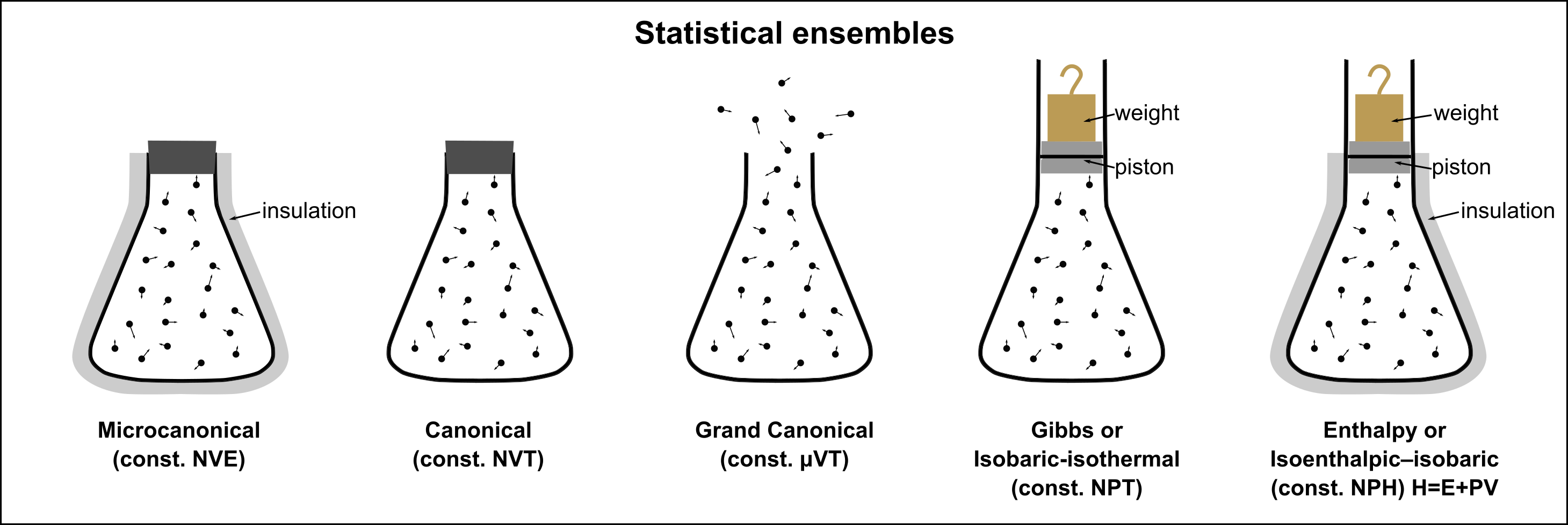
Summary of Ensembles#
Entropy as a Function of Microstate Probabilities#
Entropy is given by the Shannon-Gibbs entropy formula:
where \(p_i\) is the probability of the \(i\) th microstate.
Physical Constraints for Equilibrium#
For a system to maintain equilibrium values, the microstate probabilities must satisfy the following conditions:
Normalization:
\[ \sum_{i} p_i = 1 \]Constraint to Maintain the Expectation Value of an Observable \(X\) (e.g., Energy or Volume):
\[ \sum_{i} p_i X_i = \langle X \rangle, \quad \sum_{i} p_i Y_i = \langle Y \rangle \]
The probability of a macrostate \( (X, Y, \dots) \) follows the general form:
\[ P(X, Y, \dots) = \frac{e^{\frac{1}{k_B}S(X, Y, ..)} \cdot e^{- \beta X} \cdot e^{- \gamma Y}...}{Z} \]\[Z(\beta, \gamma, ...) = \sum_{X, Y, ...} e^{\frac{1}{k_B}S(X, Y, ..)} e^{- \beta X} e^{- \gamma Y}...\]Where \(Z\) is a normalization factor called partition function
Exponential dependence can also be seen as consequence of exchange of (energy, volume ,etc) with an environment or a large reserovoir.
Comparison of Ensembles#
Ensemble |
\( P(\text{microstate}) \) |
\( P(\text{macrostate}) \) |
|---|---|---|
Microcanonical (NVE) |
\( P(\text{microstate}) = \frac{1}{\Omega(E)} \) |
\( P(E) \sim e^{S(E)/k_B} \) (entropy-dominated) |
Canonical (NVT) |
\( P(\text{microstate}) \sim e^{-\beta E} \) |
\( P(E) \sim e^{S(E)/k_B - \beta E} \) (entropy-weighted by energy) |
Grand Canonical (µVT) |
\( P(\text{microstate}) \sim e^{\beta (\mu N - E)} \) |
\( P(N, E) \sim e^{S(N,E)/k_B + \beta (\mu N - E)} \) |
Isothermal-Isobaric (NPT) |
\( P(\text{microstate}) \sim e^{-\beta (E + PV)} \) |
\( P(E, V) \sim e^{S(E, V)/k_B - \beta (E + PV)} \) |
Entropy dependence \(e^{S/k_B}\) is universal across all ensembles.
Microstate probability follows different forms based on constraints from different thermodynamic potentials.
Macrostate probability always includes an entropy term but is modified by energy, pressure, and chemical potential, depending on the ensemble.
Extensive vs intensive variables#
The total differential of internal energy \( U \) in a thermodynamic system can be expressed in terms of its conjugate variables:
where each pair \((X_i, f_i)\) represents a conjugate extensive and intensive variable respectively, such as:
\( (S, T) \) → entropy and temperature,
\( (V, -P) \) → volume and pressure,
\( (N, \mu) \) → particle number and chemical potential,
\( (M, B) \) → magnetization and magnetic field.
Laplace Transform and Ensemble Connections#
The Laplace transform connects different thermodynamic ensembles by linking the partition function to energy and volume fluctuations. It effectively approximates a Legendre transform in the thermodynamic limit.
Canonical Ensemble (Energy Integration):
\[ Z(\beta, N, V) = \int dE \, \Omega(E) e^{-\beta E} \approx e^{\min_E [S(E)/k_B - \beta E]} \]\[ Z(\beta, N, V) = e^{-\beta [U - TS]} = e^{-\beta F(\beta, N, V)} \]Isothermal-Isobaric Ensemble (Volume Integration):
\[ Z(\beta, N, P) = \int dV \, Z(\beta, N, V) e^{-\beta P V} \approx e^{\min_V [F(V) - \beta P V]} \]\[ Z(\beta, N, P) = e^{-\beta [U - TS - PV]} = e^{-\beta G(\beta, N, P)} \]Thus, free energy functions naturally emerge as Legendre transforms of internal energy through Laplace integration over fluctuating variables.
Legendre Transform and Thermodynamic Potentials#
The Legendre transformation allows us to reformulate equilibrium conditions (e.g., entropy maximization) in terms of more convenient variables (e.g., free energy minimization).
This transformation makes it possible to work with temperature and pressure as control variables instead of entropy and volume.
Free Energies as Legendre Transforms of Internal Energy
Helmholtz Free Energy (Legendre transform over \( S \)):
Gibbs Free Energy (Legendre transform over \( S, V \)):
Partition Functions and Legendre Transforms#
The partition function naturally follows the structure of a Legendre transform, as it is related to free energy via:
The \(\Psi\) is a thermodynamic potential obtained through Legendre transformation of the internal energy.
Fluctuation-Response Relations#
For a given extensive variable \( X \) and its conjugate intensive variable \( f \), the partition function \( Z \) governs both the mean value and fluctuations of \( X \).
Mean value of \( X \) at constant \( f \):
\[ \langle X \rangle = \frac{\partial \log Z}{\partial (\beta f)} \]Fluctuations of \( X \) at constant \( Y \):
\[ \sigma^2_X = \langle X^2 \rangle - \langle X \rangle^2 = \frac{\partial^2 \log Z}{\partial (\beta f)^2} \]This relation shows that fluctuations in \( X \) are directly linked to the second derivative of the partition function, a fundamental result of statistical mechanics.
Energy fluctuations (Canonical Ensemble):#
where \( C_V \) is the heat capacity at constant volume.
Particle number fluctuations (Grand Canonical Ensemble):#
where \( \kappa_T \) is the isothermal compressibility.
Key Insights#
Fluctuations decrease as system size increases, typically scaling as \(1/\sqrt{N}\).
Response functions (e.g., heat capacity, compressibility) determine fluctuation magnitude.
Ensemble equivalence ensures that for large systems, different ensembles (canonical, grand canonical, etc.) give equivalent macroscopic results, despite differing fluctuation magnitudes.