Review of thermodynamics principles

Review of thermodynamics principles#

What you will know

Thermodynamics is an exact phenomenological theory that describes changes in material systems in equilibrium. “Phenomenological” means that macroscopic phenomena are defined in terms of a few observable and measurable variables, without reference to microscopic details.
- Extensive variables: are additive quantities such as energy, volume, and the number of moles—that completely define the thermodynamic space.
- Intensive variables: are size independent quantities such as temperature, pressure and magneitc field. These are derived from extensive variables offering convenient description of system under constant external conditions.
The central goal of thermodynamics is calculating transformations in thermodynamic space by constructing quasi-static paths which obey the fundamental laws:
- The first law expresses the conservation of energy.
- The second law determines the direction of spontaneous processes. It implies that thermodynamic space is foliated into adiabatic surfaces of constant entropy.

Extensive vs Intensive variables#

Extensive variables: Depdent on System size These are fundamental variables that uniquely define the equilibrium states. Examples are $V, N, E, S$ .
Intensive variables: Size Independent These are derived from the extensive ones and are considered as conjugate pairs. E.g $V - P$ , $N - μ$ and $S - T$ , are conjugate pairs.
Intensive variables do not have the same fundamental status as extensive variables
- Because they do not always uniquely describe the state of matter in equilibrium.
- For example, a glass of water with and without an ice cube can be under 1 atm and 0 C, whereas energy and entropy volume values will differ.

Exercise: Extensivity of Energy

For volume, it may be straightforward to explain why it is extensive. But why is Energy an extensive quantity $E = E_{1} + E_{2}$ for a system with N interacting particles?
Does extensivity of energy always hold? think of two molecules, ten, thousands, Avogadro number?

Equilibrium and thermodynamic space#

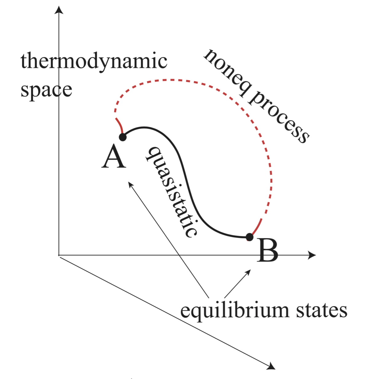
../_images/adiabat.png — Fig. 12 A and B are equilibrium states. A quasistatic process connecting A and B is in the thermodynamic space (however, see the warning in the text). From A to B a process need not be quasistatic. Then, most such processes are outside the thermodynamic space (broken curve).#

Equilibrium refers to a state of matter which is unchanging. There are no macroscopic fluxes or flows of energy or matter.
The state of Equilibrium is defined relative to observation time! A glass of water on the table is in a state of equilibrium on the time scale of minutes but in a state of non-equilibrium over the scale of days because water evaporates, changing the thermodynamic state of the glass.
Euilibrium is represented as a point in the Thermodynamic space $E (X_{1}, X_{2}, . . .)$ where $X_{i}$ are extensive variables.
- These coordinates have unique and well-defined values for each equilibrium state irrespective to how such state was created.
- Intensive variables become ill-defined if the system is not in equilibrium (temperature, pressure, etc).
- Functions like energy $E$ are called state functions, and their changes are given by differences between initial or final state only $Δ E = E_{f} - E_{i}$ .
- On the other hand one can have quantities such as work $W$ or heat $Q$ . These are path dependent characterizing the way energy is transferred to the system and not characterizing equilibrium states!

Fundamental equation of thermodynamics#

Fundmanetal Equation of Thermodynamics

E (X_{1}, X_{2} . . .)

$E (X)$ as a function of in thermodynamics of all of the extensive variables $X = X_{1}, X_{2}, . . .$ … describing the system.

Transformations between equilibrium states is the central task of thermodynamics. Knowing the fundamental equation, one can predict the equilibrium state B, which results from equilibrium state A through spontaneous transformation upon removal of a constraint. E.g computing $Δ E = E_{B} - E_{A}$ given expansion of a box.
Quasi-static path: a dense succession of equilibrium states that connects A with B in extensive variables is constructed to compute changes in thermodynamic variables between states A and B. The quasistatic process ensures the system does not deviate from the equilibrium state during transformation.
Reversible transformations can go forward or backward without any change in the environment. This necessitates the introduction of Entropy, which differentiates reversible from non-reversible changes.
The quasistatic path may or may not be reversible Just because the process is infinitely slow and locally in equilibrium does not make it reversible along the path of transofrmation. For instance, poking a small hole in a container and letting one molecule out very slowly does not make the process reversible.

First Law#

First Law of Thermodynamics

d E = δ Q + δ W

$δ Q$ and $δ W$ are inexact differentials. This means that work done to go from A to B will depend on a path from A to B
dE is an exact diffrential. This means the energy difference between states A and B is the same regardless of the path one takes.

Note on signs

By convention sign of work or heat is positive if energy is transfered to the system. Negative if it system loses energy. Hence think about signs from the perspective ofa system under study.
If engine does work against external pressure $p$ then $d W = - p d V$ . You can see work is going to be negative for expanding volume $d V > 0$ and positive for contracting $d V < 0$
If system is absorbing heat from environment (heating up) $δ Q > 0$ . If the system is refridgerating then $δ Q < 0$

Adiabatic Change $d Q = 0$

d E = d W

No work

d E = d Q

Adiabatic Processes#

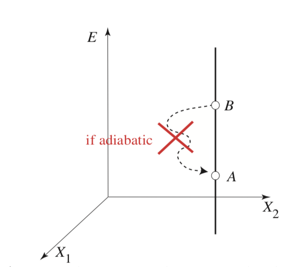
Planck’s Formulation of the Second Law

For any adiabatic process in which all work coordinates return to their initial values (i.e., a cyclic process), the energy of a thermally isolated system cannot decrease:

$Δ E \geq 0$

Intuitively, this means that when performing pure mechanical work on a system, we can only impart energy to it due to friction or dissipation. Conversely, it is impossible to “steal” energy from a closed system purely through mechanical work without any accompanying environmental change.
Consequently, not all paths in thermodynamic space are accessible; one cannot always transition freely from state A to state B. This suggests the existence of a fundamental constraint—possibly a new variable—that dictates when transitions are allowed and when they are not.

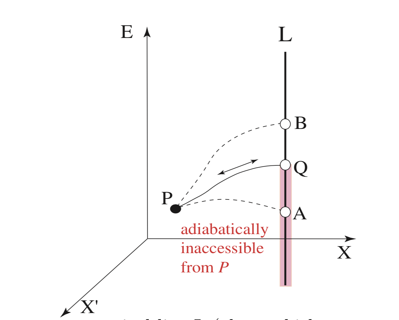
../_images/Adiabats.png — Fig. 13 Let Q be a state on a vertical line L (along which we can move with heat exchange alone) that can be reached from state P adiabatically and quasistatically. If state A can be reached by an adiabatic process from P, then adiabatically we can go from Q to A via P, violating Planck’s principle. Thus, the shaded portion is inaccessible from P adiabatically. If state B can be reached by an adiabatic and quasistatic process from P, then adiabatically we can go from B to Q via P, violating Planck’s principle, again. Thus, Q is unique: there is only one point on L that can be reached from P adiabatically and quasistatically.#

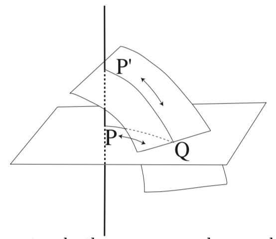
../_images/NO1.png — Fig. 14 If two adiabats cross or touch, then we can make a cycle that can be traced in any direction, because PQ and P’Q can be traced in either directions, so Planck’s principle is violated.#

This restriction implies that adiabatic surfaces (or lines) cannot intersect. If they did, one could design a cyclic mechanical process that decreases the system’s energy, violating the second law. Moreover, an intersection would imply that the same thermodynamic coordinates correspond to two different forces (energy derivatives), which is physically inconsistent.
- Therefore, thermodynamic space is foliated by non-intersecting adiabats.
- This structure naturally leads to the definition of an extensive variable, Entropy $S (E)$ , which remains constant along each adiabatic surface and increases with energy across different adiabats.
- Since entropy is a monotonic increasing function of energy $S (E)$ , it follows that Planck’s formulation implies:

Second Law for Adiabatic Processes

Δ S \geq 0

However, as we shall see the entropy-based Second Law is more general, as it applies to both adiabatic and non-adiabatic transformations.

Reversible Heat Exchange#

Moving from one adiabat to another requires heat input or removal.
This structure underlies entropy-based formulations of the Second Law, as entropy remains constant or increases in an adiabatic process.

d S = S (E + d E) - S (E) = \frac{d S}{d E} d E = \frac{d Q}{T}

Here, we identify the prefactor as the temperature, which we will soon rediscover in statistical mechanics.

T = {(\frac{d S}{d E})}^{- 1},

Since mechanical manipulation alone does not move the system between adiabats, this implies that entropy can only be reduced by cooling ( $d Q < 0$ ).

Second Law#

For general non-adiabatic case of system in contact with an infinitely large reservoir (heat bath) it is the entropy of the combined system+reservoir that must increase.

d S + d S_{r} \geq 0

The reservoir the entropy change is solely due to heat exchange $Q_{r} = - Q$

d S_{r} = \frac{δ Q_{r}}{T} = - \frac{δ Q}{T}

Second Law of Thermodynamics

d S \geq \frac{δ Q}{T}

Understanding the Signs#

Irreversibility and Entropy Production
- The inequality $d S > \frac{δ Q}{T}$ captures entropy increase due to internal irreversibilities, such as:
- Friction, viscosity, turbulence** in fluids. Non-equilibrium chemical reactions. Unrestrained (free) expansion
Reversible Heat Transfer
- The equality $d S = \frac{δ Q}{T}$ holds when:
  - The system remains in thermal equilibrium with surroundings.
  - Heat exchange occurs infinitesimally slowly (e.g., between objects with an infinitesimal temperature difference).
Equilibrium Condition:
- Entropy is maximized $d S = 0$ and no spontaneous changes occur:

Exercise: Bending an elastic sheet

Consider and elastic sheet that you do some work and bend slowly and to a good approximations reversibly hence $Δ S = 0$ and this was adiabatic process so $Q = 0$
When you release the shit it will rapidly snap back. No heat was exchanged with environment at that instant so the process is adiabatic $Q = 0$ and no work was done so $W = 0$ , yet the process ir irreversible hence $Δ S > 0$ . Explain what happened.

Gibbs Relation#

The internal energy of a thermodynamic system can be expressed as a function of its extensive variables: entropy $S$ , volume $V$ , and number of particles $N$ :

E = E (S, V, N) .

Taking the total differential of $E$ , we obtain:

d E = {(\frac{\partial E}{\partial S})}_{V, N} d S + {(\frac{\partial E}{\partial V})}_{S, N} d V + {(\frac{\partial E}{\partial N})}_{S, V} d N .

We identify the intensive variables conjugate to the extensive variables:
Temperature $T$

$T = {(\frac{\partial E}{\partial S})}_{V, N}$
Pressure $P$

$P = - {(\frac{\partial E}{\partial V})}_{S, N}$
Chemical potential $μ$

$μ = {(\frac{\partial E}{\partial N})}_{S, V}$

The first law of thermodynamics can then be written in its fundamental formm Texpressing how changes in entropy, volume, and particle number contribute to changes in energy.

Gibbs Relation

d E = T d S - P d V + μ d N .

Example: Fundamental equation of ideal gas

Consider an ideal gas in a container that is in a state of equilibrium and is therefore described by $E (S, N, V)$ or $S (E, N, V)$ fundamental equation.

Using the ideal gas relation $P V = N k_{B} T$ for monoatomic gas, derive an expression for entropy

Exercise: doubling of Volume

Consider the sudden Doubling of the volume of one mol of an ideal gas in a container.

Using information theoretical view of entropy, compute how much entropy of the system changes as a result of sudden doubling.
Using the expression for entropy, derive how much entropy of the system changes as a result of sudden doubling.
Is the adiabatic expansion of gas due to volume doubling reversible or irreversible?
Think about quasistatic path for this process

Gibbs Duhem relation#

The extensivity property implies linear scaling with respect to extensive variables. In other words, extensive variables are additive quantities.

E (λ S, λ V, λ N) = λ E (S, V, N)

Using chain rule we get a liner relationship between extensive variables not involving any differentials:

E (S, V, N) = \frac{\partial E (λ S, λ V, λ N)}{\partial λ} = (\frac{\partial E}{\partial λ S})_{V, N} S + (\frac{\partial E}{\partial λ V})_{S, N} V + (\frac{\partial E}{\partial λ N})_{S, V} N

When we take the derivative of E and compare with Gibbs relation we end up with equation where independent variables are now intensive ones

Euler Relation

E = T S - P V + μ N

Gibbs Duhem relation

S d T - V d P + N d μ = 0

Entropy Maximization Principle#

When we release a constraint in an adiabatic system the extensive coordinates $X_{i}$ change. This spontaneous change must always lead to increase in entropy $Δ S \geq 0$
Entropy can increase until reaching its maximum possible value after which no further change is possible.
A change in system entropy $δ S$ due to any change or pertrubation is therefore telling us that
- If $δ S > 0$ system spontaneously evolves
- If $δ S < 0$ system is thermodynamically stable (any change from maximum leads to decrease of entropy)
Therefore the second law gives us a variational principle in terms of entropy to find stable equilibrium states for an adiabatic systems.

Entropy Maximization Principle

The state of equilibrium is found via entropy maximization over variable constraints $X = X_{1}, X_{2}, . . .$

m a x_{X} S (E, X) \to X_{1}^{e q}, X_{2}^{e q}, . . .

Thermodynamic Stability and Concavity of Entropy#

Let us join two systems made of the same substances to make a single system. The entropy maximization principle tells us that the entropy of the resultant compound system is given by

S (E, X) = m a x [S (E_{1}, X_{1}) + S (E_{2}, X_{2})]

Where the maximum is taken over all the partitions of $E$ and $X$ (collection of any work coordinates) between the two systems as $E = E_{1} + E_{2}$ and $X = X_{1} + X_{2}$
This implies with the aid of the extensivity $S (α E, α X) = α S (E, X)$

S (α E + (1 - α) E^{'}, α V + (1 - α) V^{'}) \geq α S (E, V) + (1 - α) S (E^{'}, V^{'})

for any $α \in [0, 1]$ . That is, S is a concave function (its graph is convex upward) of all the thermodynamic coordinates

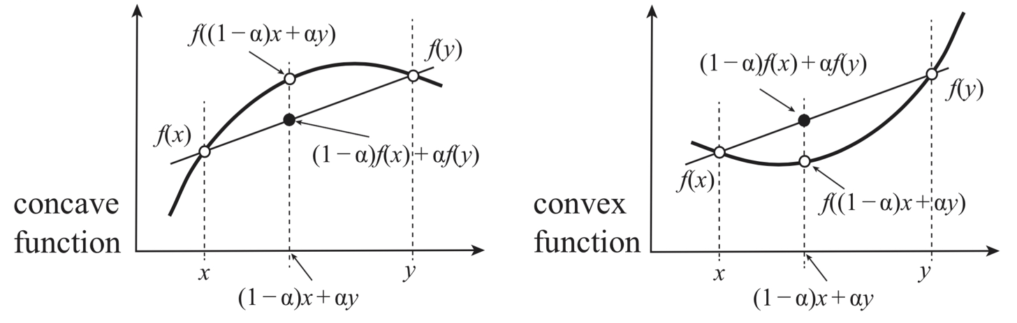
../_images/concave_convex.png — Fig. 15 Entropy is a concave function of extensive variables.#

Energy Minimization Principle

Entropy maximimization principle states that at equilibrium values of thermodynamic coordinates $X^{e q}$ $E^{e q}$ entropy is maximized so any deviation $X^{'}$ in coordinates leads to smaller entropy:

S (E^{e q}, X^{e q}) - S (E^{e q}, X^{'}) > 0

Given that entropy is an increasing function of energy we can boost the energy to $E^{'} > E^{e q}$ in the second term to get an equality

S (E^{e q}, X^{e q}) - S (E^{'}, X^{'}) = 0

This implies that under the constant entropy condition, if an extra constraint to fix $X$ is removed the system goes from higher $E^{'}$ to lower $E$ .
Thus we have Energy Minimization Principle: internal energy is minimized under a constant entropy condition, the system must be in equilibrium.

Thermodynamic stability and Heat Capacity#

The entropy function $S (E, V, N)$ must be concave to ensure stability.
Mathematically, for equilibrium stability, the second derivative of entropy must satisfy:

{(\frac{\partial^{2} S}{\partial E^{2}})}_{V, N} \leq 0

This inequality shows that equilibrium state is stable against any thermal fluctuations that deviate from equilibrium.
Taking second derivative of entropy and making use of the following equality:

\frac{1}{T} = \frac{\partial S}{\partial E}

{(\frac{\partial^{2} S}{\partial E^{2}})}_{V} = - \frac{1}{T^{2}} {(\frac{\partial T}{\partial E})}_{V} .

Since heat capacity at constant volume is:

C_{V} = {(\frac{\partial E}{\partial T})}_{V},

we obtain the stability condition:

C_{V} = - \frac{T^{2}}{{(\frac{\partial^{2} S}{\partial E^{2}})}_{V}} > 0

Implication: A positive heat capacity ( $C_{V} > 0$ ) ensures local thermodynamic stability.

Spontaneous Change and Partitioning of Extensive Variables#

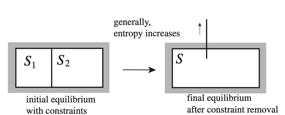
../_images/part1.png — Fig. 16 What way the system will parition energy, volume particles when the constraint separating flow of these variables is removed?#

A spontaneous process occurs when a system undergoes a transformation that maximizes entropy. In thermodynamic equilibrium, extensive variables (such as energy, volume, and particle number) partition between subsystems in a way that maximizes the total entropy.
Consider two subsystems, $I$ and $I I$ , exchanging energy. Since the total energy is conserved we can write down total energy and entropy as:

$E = E_{I} + E_{I I}$

$S_{tot} (E) = S_{I} (E_{I}) + S_{I I} (E - E_{I})$
At equilibrium, entropy is maximized by varying in this case the only free extensive coordinate $E_{I}$ , which determines energy partitioning:

$δ S_{tot} (E) = \frac{\partial S_{I}}{\partial E_{I}} δ E_{I} - \frac{\partial S_{I I}}{\partial E_{I I}} δ E_{I} = 0$

$\frac{\partial S_{I}}{\partial E_{I}} = \frac{\partial S_{I I}}{\partial E_{I I}}$
We once again come to appreciate that derivative of entropy with respect to energy is related to temperature:

$\frac{1}{T} = \frac{\partial S}{\partial E}$
- We obtain the equilibrium condition showing that temperature imbalance drives energy distirbution until we reach equal temperatures throughout the system.
$T_{I} = T_{I I}$
In general system spontaneously evolves toward equilibrium by redistributing energy, volume, and particles:

In equilibrium intensive vairables are equal throughout the system

Temperature drives energy partitioning

T_{I} = T_{I I}

Pressure drives volume partitioning

P_{I} = P_{I I}

Chemical potential drives particle partitioning

μ_{I} = μ_{I I}

Example: find final energy partitioning

The fundamental equations for two systems $A$ and $B$ separated by diathermal wall (no heat flow allowed) is

S = {(N V U)}^{1 / 3}

The total energy is $U_{A} + U_{B} = 80 J$
The volume and mole number of system $A$ are $9 \times 10^{- 6} m^{3}$ and $3$ mol respectively.
The volume and mole number for system $B$ are $4 \times 10^{- 6} m^{3}$ and $2$ mol respectively.

Plot the total entropy $S_{A} + S_{B}$ as function of energy distribution between two systems $X = U_{A} / (U_{A} + U_{B})$
If we enable heat flow between systems A and B a new equilibrium state would be established. What would $U_{A}$ and $U_{B}$ be like in this new equilibrium state?

Appendix#

Entropy and Efficiency of Heat Engines

Consider a heat engine that absorbs heat $Q_{H}$ from a hot reservoir, performs work $W$ , and rejects heat $Q_{C}$ to a cold reservoir.
The total energy of the system (engine + reservoirs) is conserved. Using the first law of thermodynamics, we express this as:

Δ E = Q_{H} - Q_{C} - W = 0

Since the engine does work on the surroundings, it loses energy, meaning $W$ is considered and negative from the system’s perspective. To express work as a positive quantity:

| W | = | Q_{H} | - | Q_{C} |

The efficiency of the engine, defined as the fraction of input heat converted into useful work, is:

η = \frac{| W |}{| Q_{H} |} = 1 - \frac{| Q_{C} |}{| Q_{H} |}

The second law of thermodynamics states that total entropy must increase or remain constant:

Δ S_{total} = Δ S_{H} + Δ S_{C} \geq 0

Since entropy is a state function, we write:

Δ S_{H} = - \frac{| Q_{H} |}{T_{H}}, Δ S_{C} = \frac{| Q_{C} |}{T_{C}}

\frac{| Q_{C} |}{T_{C}} \geq \frac{| Q_{H} |}{T_{H}}

This inequality shows that an irreversible engine dissipates more heat to the cold reservoir, leading to lower work output.
Substituting this result into the efficiency expression:

η = 1 - \frac{| Q_{C} |}{| Q_{H} |}

yields the fundamental upper bound on efficiency:

η \leq 1 - \frac{T_{C}}{T_{H}}

This result represents the Carnot efficiency, which is the maximum possible efficiency for any heat engine operating between two reservoirs at temperatures $T_{H}$ and $T_{C}$ .

Practical symmary of thermodynamic principles

1.Thermodynamic variables are either extensive or intensive. The total amount of an extensive quantity of a compound system is the sum of the extensive quantities of the subsystems (additivity)

There is a state called an equilibrium state. which is described in terms of extensive thermodynamic coordinates ( $E$ , $X_{1}$ , $X_{2}$ ), where $E$ is the internal energy and $X_{i}$ are coordinates in thermodynamic space.
The conservation of energy: $d E = δ Q + δ W = δ Q - \sum x_{i} d X_{i}$ where the variables appear in intensive-extenisve “conjugate pairs” like $(- P, V), (μ, N), (x, X)$
The thermodynamic space is foliated into $S = c o n s t$ (hyper) surfaces. For adiabatic process with work only, $Δ S < 0$ never happens; to reduce entropy we definitely need cooling.
A reverisble heat transfer increases entropy of system by $d S = \frac{δ Q}{T}$ amount.
Thermodynamics calculations proceed by defining a quasistatic process for which Gibbs relation holds: $d E = T d S - p d V + μ d N + . . .$ often it is convenient to write $d S = \frac{1}{T} d E + \frac{p}{T} d V + μ d N$

Problems#

Problem 1 Fundamental equations#

The following ten equations are purported to be fundamental equations for various thermodynamic systems. Five, however, are inconsistent with the basic postulates of a fundamental equation and are thus unphysical. For each, plot the relationship between $S$ and $U$ and identify the unacceptable five. $v_{0}$ , $θ$ , and $R$ are all positive constants and, in the case of fractional exponents, the real positive root is to be implied.

$S = {(\frac{R^{2}}{v_{0} θ})}^{1 / 3} {(N V U)}^{1 / 3}$
$S = {(\frac{R}{θ^{2}})}^{1 / 3} {(\frac{N U}{V})}^{2 / 3}$
$S = {(\frac{R}{θ})}^{1 / 2} {(N U + \frac{R θ V^{2}}{v_{0}^{2}})}^{1 / 2}$
$S = (\frac{R^{2} θ}{v_{0}^{3}}) \frac{V^{3}}{N U}$
$S = {(\frac{R^{3}}{v_{0} θ^{2}})}^{1 / 5} (N^{2} U^{2} V)$
$S = N R \ln (\frac{U V}{N^{2} R θ v_{0}})$
$S = {(\frac{N R U}{θ})}^{1 / 2} \exp (- \frac{V^{2}}{2 N^{2} v_{0}^{2}})$
$S = {(\frac{N R U}{θ})}^{1 / 2} \exp (- \frac{U V}{N R θ v_{0}})$
$U = (\frac{N R θ V}{v_{0}}) (1 + \frac{S}{N R}) \exp (- S / N R)$
$U = (\frac{v_{0} θ}{R}) \frac{S^{2}}{V} \exp (S / N R)$

Problem 2: Expansion of gas into the vacuum#

As a general case of gas expanding into the vacuum, use the Gibbs relation for $E$ to show that $(\frac{\partial S}{\partial V})_{E} > 0$ this would show that free adiabatic expansion is accompanied by entropy increase and is hence and irreversible process.
Now consider a gas in container energy described by the following equation $E = 3 / 2 N k T - N^{2} V / a$
- Plot E as a function of V for a few temperatures.
- Suppose that a gas expands adiabatically into a vacuum. How will the energy and entropy of the system change, and what is the work done by the gas?
- Initially, the gas occupies a volume $V_{1}$ at a temperature $T_{1}$ . The gas then expands adiabatically into a vacuum to occupy a total volume $V_{2}$ . What is the final temperature $T_{2}$ of the gas?

Problem 3 Entropy of mixing two gases#

Using the expression for an ideal gas $S = N k_{B} l o g \frac{V}{N}$ , calculate the entropy change resulting after removing a divider separating $N_{A}$ molecules of gas A occupying Volume $V_{A}$ from $N_{B}$ molecules of gas B occupying volume $V_{B}$ .

Hints

The system overall is thermally insulated and pressure and temperatures are constant; hence, numbers and volumes are proportional $N_{A} \sim V_{A}$ so you can express entropy change entirely in terms of molar numbers or their fractions $x_{A} = N_{A} / (N_{A} + N_{B})$
You need to first calculate the entropy change due to gas A expanding from volume $V_{A}$ to volume $V = V_{A} + V_{B}$ and the same for gas B. the total entropy change will be the sum of these two changes.

Problem 4: Entropy of heating#

1 kg of water (specific heat = 4.2 kJ/(kg·K)) at $0^{o} C$ is in contact with a $50^{o} C$ heat bath, and eventually reaches $50^{o} C$ . What is the entropy change of the water? What is the increase of the entropy of this water plus the heat bath?
Imagine now that the water at $0^{o} C$ is in contact with a $25^{o} C$ heat bath. Then, after reaching thermal equilibrium, the water is subsequently put in contact with a $50^{o} C$ heat bath until it reaches the final temperature $50^{o} C$ . What is the increase of the entropy of the water after it has been put in contact with two heat baths? Compare the answer to the case of (1)
Show that in the two-step heating process, whatever the first heat bath temperature T is between $0^{o} C$ and $50^{o} C$ , the total change of entropy of the water plus heat baths is less than the case of (1)