Mean Field Theory#
Mean Field Approximation replaces fluctuating terms with their averages. For a function dependent on multiple variables, the approximation removes all correlations between variables:
Mean field approximation is widely used in electronic-structure theory (Hartree-Fock), theory of liquids (Van der Waals) and condensed matter physics.
Application of MFA to the Ising Model
In the Ising model, this approximation allows us to decouple spins, simplifying the system to a single parameter: the average magnetization per spin, \(m\).
The 1/2 avoids double counting, and (\(q\)) denotes the number of nearest neighbors, 4 for a 2D lattice and 6 for a 3D lattice.
Detailed derivation of Mean Field Approximation of Hamiltonian
Consider the 2D Ising model where each spin \(( s_i \)) interacts with an effective field generated by its nearest neighbors (summed over \(\delta\) ):
Where the Hamiltonian field of spin \(i\) is
Now, we make a critical approximation by assuming each spin experiences an average field independent of others:
Taking average and taking care not to double count we arrive at the expression for average energy obtained before.
Self-Consistent Equation
Partition function Since we decoupled each spin partition function is a product of the partition function of individual spins \(Z=z^N\), and we only have to microstates for each spin \(s_i=\pm1\)
Average Spin Orientation: The mean spin orientation, given the probabilities, is then:
We see that the hyperbolic tangent arises from the balance of probabilities for spin orientations under the influence of the mean field.
Free energy of mean field ising models#
Defining macrostate M
Consider \(N\) spin-lattice macrostates with magnetization value \(M\) resulting from a net number of spins pointing up (down).
Dividing by N we can express probabilities of spin up and down \(N_{\pm}/N\) in terms of magnetization per spin \(m=M/N\) $\(p_{\pm} = \frac{1\pm m}{2}\)$
Entropy, Energy, and Free energy
Entropy is the familiar \(S = -\sum_i p_i\log p_i\) expression where \(p_i\) is spin up and down probabilities.
Energy for total spin magnetization \(M\) is the N times the average energy of each spin in the mean-field approximation
Free energy
Dimensionless free energy per particle
Finding critical point \(Tc\)
Magnetization as a function of temperature
The equilibrium value of magnetization is found by minimizing free energy. By taking the first derivative of free energy, we end up with an equation that can only be solved in a self-consistent manner by starting with a guess and iterating until both sides of the equation are equal.
For \(h=0\) we have the following simple equation to be solved in self consistent manner:
For small values of \(m\), we can make an approximation by taylor expanding \(tanh^{-1}(x) = x+1/3x^3\)
For \(h = 0\) case the solution is either trivial \(m=0\) or we get:
Investigating various limits#
The \(h=0\) MFA case
The equation can be solved in a self-consistent manner or graphically by finding intersection between:
\(m =tanh(x)\)
\(x = \frac{Jqm}{k_BT}\)
When the slope is equal to one it provides a dividing line between two behaviours.
MFA shows phase transitio for 1D Ising model at finite \(T=T_c\)!
import ipywidgets as widgets
from ipywidgets import interactive, interact
import matplotlib.pyplot as plt
import numpy as np
# Constants
J = 1  # Interaction strength
k = 1  # Boltzmann constant (set to 1 for simplicity)

def entropy(m):
    # Handle log of zero by adding a small number to the argument
    small_number = 1e-10
    return -(1+m)/2 * np.log((1+m)/2 + small_number) - (1-m)/2 * np.log((1-m)/2 + small_number)

def free_energy(m, T):
    # Calculate the free energy for given m and T
    return -0.5 * J * m**2 - T * entropy(m)

def plot_free_energy(T):
    # Magnetization range
    m_values = np.linspace(-1, 1, 100)
    F_values = [free_energy(m, T) for m in m_values]

    # Plotting
    plt.figure(figsize=(8, 5))
    plt.plot(m_values, F_values, label=f'T = {T}')
    plt.xlabel('Magnetization (m)')
    plt.ylabel('Free Energy per Spin (F)')
    plt.title('Mean-field Free Energy vs. Magnetization')
    plt.legend()
    plt.grid(True)
    plt.show()

interactive(plot_free_energy, T=(0.1, 2, 0.1 ))
def mfa_ising_Tc(T=1, Tc=1):

    x  = np.linspace(-3,3,1000)

    f = lambda x: (T/Tc)*x
    m = lambda x: np.tanh(x)

    plt.plot(x,m(x), lw=3, alpha=0.9, color='green')

    plt.plot(x,f(x),'--',color='black')
    idx = np.argwhere(np.diff(np.sign(m(x) - f(x))))
    plt.plot(x[idx], f(x)[idx], 'ro')

    plt.legend(['m=tanh(x)', 'x'])

    plt.ylim(-2,2)
    plt.grid('True')
    plt.xlabel('m',fontsize=16)
    plt.ylabel(r'$tanh (\frac{Tc}{T} m )$')
    plt.show()
interact(mfa_ising_Tc, T=(0.1,5))
<function __main__.mfa_ising_Tc(T=1, Tc=1)>
def mfa_ising_h_vs_m(T=1):

    Tc = 1
    x  = np.linspace(-1,1,200)

    h = T*(np.arctanh(x) - (Tc/T)*x)

    plt.plot(x, h, lw=3, alpha=0.9, color='green')

    plt.plot(x, np.zeros_like(x), lw=1, color='black')
    plt.plot(np.zeros_like(x), x, lw=1, color='black')

    plt.grid(True)

    plt.ylabel('m',fontsize=16)
    plt.xlabel('h',fontsize=16)
    plt.ylim([-1,1])
    plt.xlim([-1,1])
    plt.show()
interactive(mfa_ising_h_vs_m, T=(0.1,5))
import plotly.graph_objects as go
import numpy as np
from scipy.optimize import fsolve
from scipy.optimize import root_scalar  # Importing root_scalar

def compute_xcross(T, h_over_T):

    def f(M):
        Tc = 1.0  # Normalized temperature
        h = h_over_T * T  # Compute actual h from h/T and T
        return M - np.tanh((M + h) / (T / Tc))

    # Using symmetric interval for root finding to allow negative solutions
    interval = [-2.0, 2.0]

    # Check if a root is likely within the given range
    if f(interval[0]) * f(interval[1]) > 0:
        return 0.0  # If no root likely, return 0

    # Find the root using bisection method within the specified range
    result = root_scalar(f, bracket=interval, method='bisect')

    return result.root

# Define ranges for h/T  and T/Tc (from 0.2 to 1.5)
h_over_T_values = np.linspace(-0.2, 0.2, 101)
T_over_Tc_values = np.linspace(0.1, 1.6, 101)

# Create a meshgrid for T/Tc and h/T
H_over_T, T_over_Tc = np.meshgrid(h_over_T_values, T_over_Tc_values)

# Initialize an array for magnetizations
Magnetizations = np.zeros_like(H_over_T)

# Compute M for each (h/T, T/Tc) pair in the meshgrid
for i, T in enumerate(T_over_Tc_values):
    for j, h in enumerate(h_over_T_values):

        Magnetizations[i, j] = compute_xcross(T, h)


# Create a 3D surface plot using Plotly
fig = go.Figure(data=[go.Surface(z=Magnetizations, x=H_over_T, y=T_over_Tc,
                                 colorscale='RdBu',
                                 contours={
                                     #'z': {'show': True, 'start': -1.0, 'end': 1.0, 'size': 0.1, 'color':'orange'},
                                     'x': {'show': True, 'start': -1, 'end': 1, 'size': 0.05, 'color':'black'},
                                     'y': {'show': True, 'start': 0.5, 'end': 1.5, 'size': 0.1, 'color':'black'}
                                 })])

# Update plot layout
fig.update_layout(
    title='3D Plot of Magnetization M vs normalized temperature and field; T/Tc and h/T',
    scene=dict(
        xaxis_title='h/T',
        yaxis_title='T/Tc',
        zaxis_title='M',
        aspectmode='manual',
        yaxis_autorange='reversed',  # Reverse the Y-axis
        aspectratio=dict(x=2, y=2, z=0.75),  # Adjust these values as needed
        camera=dict(
            eye=dict(x=-4, y=-2, z=2),  # Adjust camera "eye" position for better view
            up=dict(x=0, y=0, z=1)  # Ensures Z is up
        )
    ),
    autosize=False,
    width=900,
    height=900
)

# Display the figure with configuration options
fig.show()
len(h_over_T_values)//2+1
51
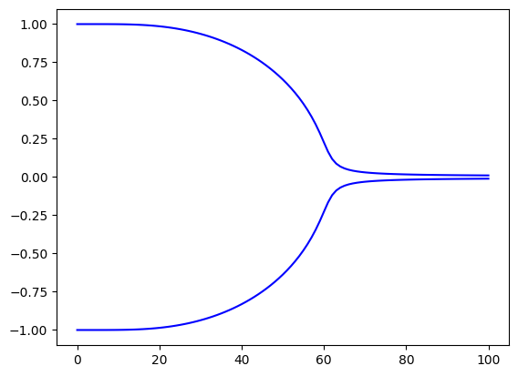
plt.plot(Magnetizations[:, len(h_over_T_values)//2-1], color='blue')
plt.plot(Magnetizations[:, len(h_over_T_values)//2+1], color='blue')
[<matplotlib.lines.Line2D at 0x180bcedf0>]
Critical exponents#
A signature of phase transitions of second kind or critical phenomena is the universal power law behaviour near critical point
Correlation lengths \(\xi\) diverge at critical points
Mean field exponents#
We can derive the value of critical exponent \(\beta\) within mean field approximation by Taylor expanding the hyperbolic tangent
One solution is obviously m = 0 which is the only solution above \(T_c\)
Below \(T_c\) the non-zero solution is found \(m=\sqrt{3}\frac{T}{T_c} \Big(1-\frac{T}{T_c} \Big)^{1/2}+...\)
\(\beta_{MFA}=1/2\)
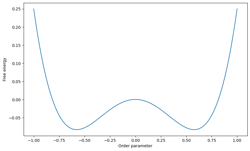
Landau theory#
# Calculate the free energy for different temperatures
T = 5
a, b = -1, 3

phi = np.linspace(-1, 1, 100)
F   = a * phi**2 / 2 + b * phi**4 / 4

# Plot the free energy as a function of the order parameter for different temperatures
plt.figure(figsize=(10, 6))
plt.plot(phi, F )
plt.xlabel('Order parameter')
plt.ylabel('Free energy')
plt.show()
Problems#
Use Transfer matrix method to solve general 1D Ising model with \(h = 0\) (Do not simply copy the solution by setting h=0 but repeat the derivation :)
Plot temperature dependence of heat capacity and free energy as a function for \((h=\neq, J\neq 0)\) \((h=0, J\neq 0)\) and \((h=\neq, J\neq \neq)\) cases of 1D Ising model. Coment on the observed behaviours.
Explain in 1-2 sentences:
why heat capacity and magnetic susceptibility diverge at critical temperatures.
why correlation functions diverge at a critical temperature
why are there universal critical exponents.
why the dimensionality and range of intereactions matters for existance and nature of phase transitions.
why MFT predictions fail for low dimensionsal systems but consistently get better with higher dimensions?
Using mean field approximation show that near critical temperature magnetization per spin goes as \(m\sim (T_c-T)^{\beta}\) (critical exponent not to nbe confused with inverse \(k_B T\)) and find the value of \beta. Do the same for magnetic susceptibility \(\chi \sim (T-T_c)^{-\gamma}\) and find the value of \(\gamma\)
Consider a 1D model given by the Hamiltonian:
where \(J>1\), \(D>1\) and \(s_i =-1,0,+1\)
Assuming periodic boundary codnitions calcualte eigenvalues of the transfer matrix
Obtain expresions for internal energy, entropy and free energy
What is the ground state of this model (T=0) as a function of \(d=D/J\) Obtain asymptotic form of the eigenvalues of the transfer matrix in the limit \(T\rightarrow 0\) in the characteristic regimes of d (e.g consider differnet extereme cases)