Statistical mechanics of fluids#
Classical parition function of fluids#
For a homogenous fluid particles partition function using classical Hamiltonian expression is an integral over phase space volume with two key quantum corrections:
\(N!\) accounting for indistinguishability
\(h^N\) setting the elementary unit of phase space volume
For a system composed of three types A B and C for instance the partion function would be:
With \(N=N_A+N_B+N_C\)
General exprssion of probability distribution of fluids in phase space#
The probability of a state in a classical fluid system is \(f(x^N, p^N)\)
Momentum and position coordinates are separated thanks to the form of kinetic and potential energy terms
Maxwell-Boltzmann distribution for single particles#
Momentum distribution further factorizes into sum of single particle kinetic energies:
Note that \(p^2_i = p^2_x+p^2_y+p^2_z\) and \(\phi(p_i)\). The momentum or velocity distribution is known as Maxwell-Boltzmann distribution.
For both ideal gas and real fluids Maxwell-Boltzmann distribution of velocities holds true. The difference between the systems boils down to a difference in potential energy
Configurational partition function#
Pressure is related to Free energy as
Volume dependence of partition function is in the integration limits! As volume grows, so does partition function. Therefore p is always positive. We can thus conclude that in equilibrium pressure is always a positive quantity
Thermal wavelength and broad validity of classical picture of fluids#
Classical mechanics is valid as long as De Broglie wavelength is small compared to intermolecular length scales
For a dilute gas, relevant lengths are \(\rho^{-1/3}\) (typical distance) and \(\sigma\) (diamater of particles)
\(\lambda_T < \sigma \) (classical regime is good)
\(H_2O\) vs \(D_2O\) melting and freezing points#
Classical descirption predicts configurational parition function to be independent of paritcle masses. Hence equation of state \(p = p(\beta, \rho)\) is independent of masses.
Thus if translationa, rotational and virbational degrees of freedo are well described by classical mechanics, \(H_2O\) and \(D_2O\) will have the same equation of state. Experiments however predict desnity maximum \(\rho(T)\) at \(p=1 atm\) at 4 C for \(H_2O\) and 10C in \(D_2O\). The freezing point is higher for \(D_2 O\) as well
Water is a weird fluid. Size is about \(3 A\) and thermal wavelength is around \(0.3 A\). The role of quantum fluctuations is to blurr the positions of water molecules. As the atomic mass increases, bluring goes down and fluids gets ordered. This is why \(D_2 O\) ice melts at a higher temperature, e.g need to supply more energy to disrupt the order.
Reduced configruational distribution functions#
Hard fact: \(P(r^N)\) and Q do not factorize because of inteparticle interactions with stronger interactions implying stronger correlations in positions.
Probability of many-body systems: to find particle \(1\) at \(r_1\), \(2\) and \(r_2\) …:
Marginal(ized) probability
Marginal(ized) probability for any particle 1 and 2
Radial distribution function (RDF)#
For an isotropic fluid, we have one point probability density:
The joint distribution for an ideal gas:
To measure the degree of spatial correlations, we introduce the Radial Distribution function (RDF):
RDF for isotropic fluids is due to translational invariance depends only on distance between particles:
Meaning of RDF
Since \(\rho = \rho^{1/N}\), the conditional probability density of finding a particle at r distance away from a tagged particle at the origin is:
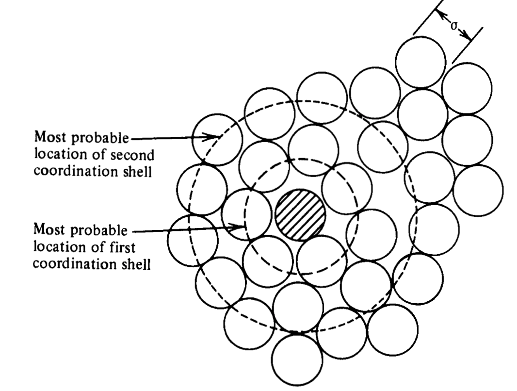
\(\rho g(r)\) is then average density of particles at distance r given that a tagged particle is at the origin
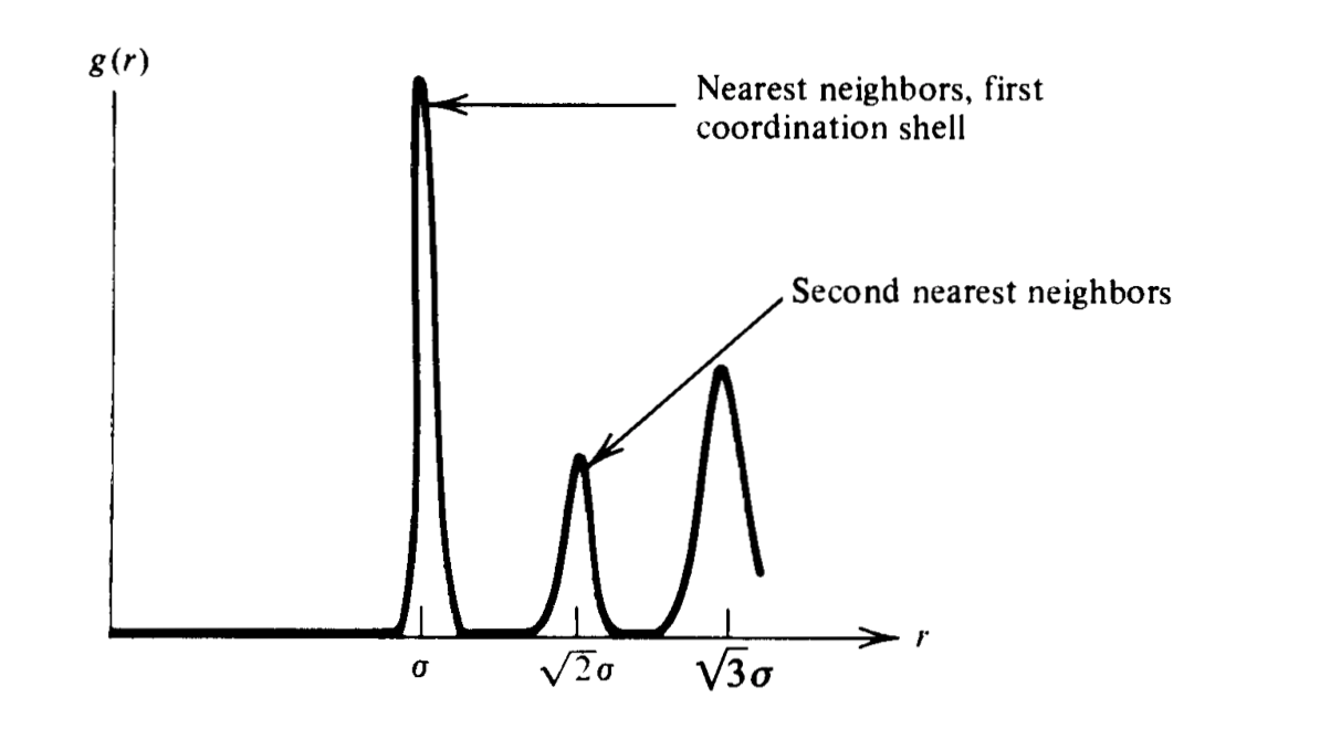
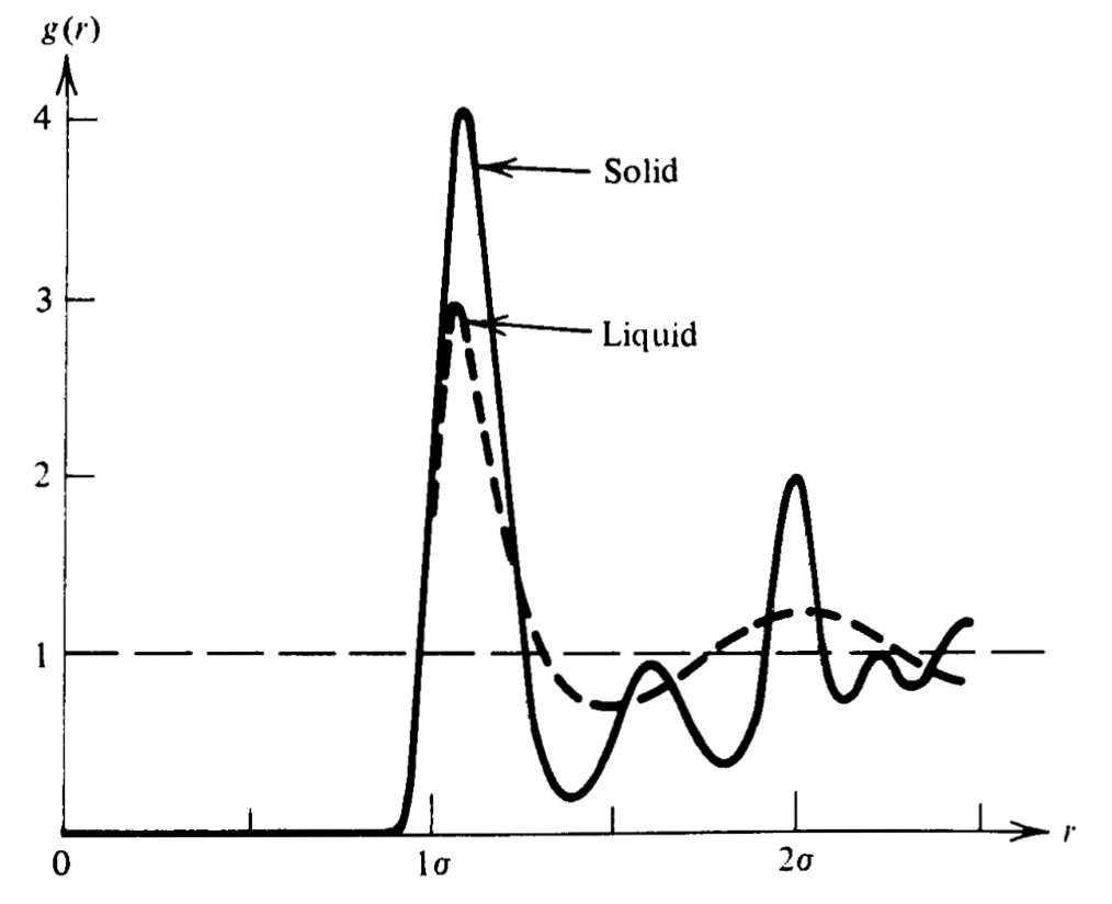
Coordination shells and structure in fluids#

Reversible work theorem and potential of mean force#
\(w(r)\) Reversible work to bring two particles from infinity to distance r
\(g(r)\) Radial distribution function