Molecular Dynamics#
import matplotlib.pyplot as plt
import ipywidgets as widgets
import numpy as np
import plotly.express as px

Is MD just Newton’s laws applied on big systems?#
Not quite: Noble prize in Chemistry 2013 just for MD
Classical molecular dynamics (MD) is a powerful computational technique for studying complex molecular systems.
Applications span wide range including proteins, polymers, inorganic and organic materials.
Alos molecular dynamics simulation is being used in a complimentary way to the analysis of experimental data coming from NMR, IR, UV spectroscopies and elastic-scattering techniques, such as small angle scattering or diffraction.
Timescales and Lengthscales#
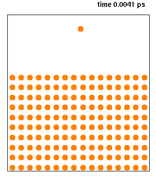
Classical Molecular Dynamics can access a hiearrchy of time-scales from pico seconds to microseconds.
It is also possible to go beyond the time scale of brute force MD byb emplying clever enhanced sampling techniques.
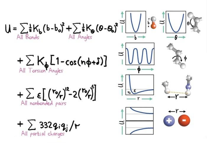
Energy function (force fields) used in classical MD#
Non-bonded interactions: Van der Waals#
@widgets.interact(sig=(1,2, 0.1),eps=(0.1,3))
def plot_lj(sig=1, eps=1):

    r  = np.linspace(0.5, 3, 1000)
    lj = 4 * eps *  ( (sig/r)**12 -(sig/r)**6 )

    plt.plot(r, lj, lw=3)
    plt.plot(r, -4*eps*(sig/r)**6, '-',lw=3)
    plt.plot(r,  4*eps*(sig/r)**12,'-',lw=3)

    plt.ylim([-3,3])
    plt.xlabel(r'$r$')
    plt.ylabel(r'$U(r)$')
    plt.legend(['LJ', 'Attr-LJ','Repuls-LJ' ])
    plt.show()
@widgets.interact(kappa=(0.1,5))
def plot_lj(kappa=0.1):

    r    = np.linspace(1, 5, 1000)

    E_DH = np.exp(-kappa*r)/r

    plt.plot(r, E_DH, lw=3)

    plt.ylim([0,1])
    plt.legend(['Debye-Huckel potential'])
    plt.xlabel(r'$r$')
    plt.ylabel(r'$U(r)$')

    plt.grid(True)
    plt.show()
@widgets.interact(kappa=(0.1,5))
def plot_harmonic(k=0.1):

    r    = np.linspace(1, 5, 1000)

    plt.grid(True)
    plt.show()
Integrating equations of motion#
No thanks, Euler#
The simplest integrating scheme for ODEs is the Euler’s method. Given the \(n\)-dimensional vectors from the ODE standard form. the Euler rule amounts to writing down equation in finite difference form.
Much better integrators are known under the names of Runge Kutta, 2nd, 4th, 6th … order
def euler(y, f, t, h):
    """Euler integrator: Returns new y at t+h.
    """
    return y + h * f(t, y)

def rk2(y, f, t, h):
    """Runge-Kutta RK2 midpoint"""

    k1 = f(t, y)
    k2 = f(t + 0.5*h, y + 0.5*h*k1)

    return y + h*k2

def rk4(y, f, t, h):
    """Runge-Kutta RK4"""

    k1 = f(t, y)
    k2 = f(t + 0.5*h, y + 0.5*h*k1)
    k3 = f(t + 0.5*h, y + 0.5*h*k2)
    k4 = f(t + h, y + h*k3)

    return y + h/6 * (k1 + 2*k2 + 2*k3 + k4)
Verlet algortihm#
Taylor expansion of position \(\vec{r}(t)\) after timestep \(\Delta t\) we obtain forward and backward Euler schems
In 1967 Loup Verlet introduced a new algorithm into molecular dynamics simulations which preserves energy is accurate and efficient.
Summing the two taylor expansion above we get a updating scheme which is an order of mangnitude more accurate
Velocity is not needed to update the positions. But we still need them to set the temperature.
Terms of order \(O(\Delta t^3)\) cancel in position giving position an accuracy of order \(O(\Delta t^4)\)
To update the position we need positions in the past at two different time points! This is is not very efficient.
Velocity Verlet updating scheme#
A better updating scheme has been proposed known as Velocity-Verlet (VV) which stores positions, velocities and accelerations at the same time. Time stepping backward expansion \(r(t-\Delta t + \Delta t)\) and summing with the forward Tayloer expansions we get Velocity Verlet updating scheme:
Substituting forces \(a=\frac{F}{m}\) instead of acelration we get
Velocity Verlet Algorithm#
1. Evaluate the forces by plugging initial positions into force-field
2. Position update:
3. Partial update of velocity
3. Force/acceleration evalutation at a new position
4. Full update of velocity
Alternative implementaitons of VV#
There is an identical to Velocity Verlet integration scheme known as the Leapfrog algorithm. which differens in the way of implementation.
In the Leap-frog velocities are calculated at half-timestep \(\Delta t/2\).
One disadvantage of the leap frog approach is that the velocities are not known at the same time as the positions, making it difficult to evaluate the total energy (kinetic + potential) at any one point in time.
def velv(y, f, t, h):
    """Velocity Verlet for solving differential equations.
    A little inefficient since same force (first and last) is evaluated twice!
    """

    # 1. Evluate force
    F = f(t, y)

    # 2, Velocity partial update
    y[1] += 0.5*h * F[1]

    # 3. Full step position
    y[0] += h*y[1]

    # 4. Force re-eval
    F = f(t+h, y)

    # 5. Full step velocity
    y[1] += 0.5*h * F[1]

    return y
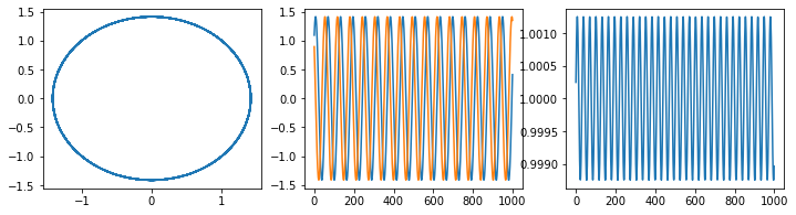
Comparison of RK and Verlet#
def f(t, y):
    ''' Define a simple harmonic potential'''

    return np.array([y[1], -y[0]])
y  = np.array([1., 1.])
pos, vel = [], []
t  = 0
h = 0.1

for i in range(1000):

    y = velv(y, f, t, h) # Change integration method venv, euler, rk2, rk4

    t+=h

    pos.append(y[0])
    vel.append(y[1])

fig, ax = plt.subplots(ncols=3, nrows=1, figsize=(12,3))

pos, vel =np.array(pos), np.array(vel)
ax[0].plot(pos, vel)
ax[1].plot(pos)
ax[1].plot(vel)
ax[2].plot(0.5*pos**2 + 0.5*vel**2)
[<matplotlib.lines.Line2D at 0x7f99a0eb0460>]
Ensemble averages#
Ensemble vs time average and ergodicity#
Kinetic, Potential and Total Energies#
Kinetic, potential and total energies are flcutuation quantities in the Molecualr dynamics simulations.
Energy conservation should still hold: The mean of total energy should be stable
Temperature#
According to equipariting result of equilibrium statistical mechanics in the NVT ensmeble
Pressure#
The microscopic expression for the pressure can be derived in the NVE ensemble using
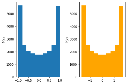
Molecular Dynaamics of Classical Harmonic Oscillator#
NVE#
def time_step_1D(pos, vel, F, en_force):
    '''Velocity Verlet update of velocities, positions and forces
    pos         (float):      position
    vel         (float):      velocity
    F           (float):        force
    en_force (function): a function whichb computes potential energy and force (derivative)
    '''

    vel   += 0.5 * F * dt

    pos   += vel * dt

    pe, F  = en_force(pos)

    vel   += 0.5 * F * dt

    return pos, vel, F, pe
def md_nve_1d(x, v, dt, t_max, en_force):
    '''Minimalistic MD code applied to a harmonic oscillator'''

    times, pos, vel, KE, PE  = [], [], [], [], []

    #1. Intialize force
    pe, F = en_force(x)

    for step in range(int(t_max/dt)):

        x, v, F, pe = time_step_1D(x, v, F, en_force)

        pos.append(x), vel.append(v), KE.append(0.5*v*v), PE.append(pe)

    return np.array(pos), np.array(vel), np.array(KE), np.array(PE)
#----parameters of simulation----
k     = 3
x0    = 1
v0    = 0
dt    = 0.01 * 2*np.pi/np.sqrt(k) #A good timestep determined by using oscillator frequency
t_max = 1000

def ho_en_force(x, k=k):
    '''Force field of harmonic oscillator:
    returns potential energy and force'''

    return k*x**2, -k*x
pos, vel, KE, PE = md_nve_1d(x0, v0, dt, t_max, ho_en_force)
fig, ax =plt.subplots(ncols=2)

ax[0].hist(pos);
ax[1].hist(vel, color='orange');
ax[0].set_ylabel('P(x)')
ax[1].set_ylabel('P(v)')

fig.tight_layout()
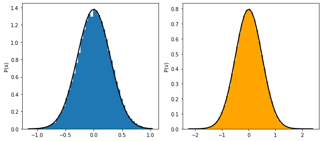
Molecualr Dynamics of Harmonic oscillator (NVT)#
Newton’s equation of motion
Langevin equation
Overdamped Langevin equation, \(m\dot{v} =0\)
Fluctuation-dissipation theorem
Velocity updating when coupled to a thermal heat bath
def langevin_md_1d(x, v, dt, kBT, gamma, t_max, en_force):
    '''Langevin dynamics applied to 1D potentials
    Using integration scheme known as BA-O-AB.
    INPUT: Any 1D function with its parameters
    '''

    times, pos, vel, KE, PE  = [], [], [], [], []

    t = 0
    for step in range(int(t_max/dt)):

        #B-step
        pe, F = en_force(x)
        v    += F*dt/2

        #A-step
        x += v*dt/2

        #O-step
        v = v*np.exp(-gamma*dt) + np.sqrt(1-np.exp(-2*gamma*dt)) * np.sqrt(kBT) * normal()

        #A-step
        x +=  v*dt/2

        #B-step
        pe, F = en_force(x)
        v    +=  F*dt/2

        ### Save output
        times.append(t), pos.append(x), vel.append(v), KE.append(0.5*v*v), PE.append(pe)

    return np.array(times), np.array(pos), np.array(vel), np.array(KE), np.array(PE)
# Ininital conditions
x     = 0.1
v     = 0.5

# Input parameters of simulation
kBT   = 0.25
gamma = 10
dt    = 0.01
t_max = 10000
freq  = 10

times, pos, vel, KE, PE = langevin_md_1d(x, v, dt, kBT, gamma, t_max, ho_en_force)
def gaussian_x(x, k, kBT):
    return  np.exp(-k*(x**2)/(2*kBT)) / np.sqrt(2*np.pi*kBT/k)

def gaussian_v(v, kBT):
    return  np.exp(-(v**2)/(2*kBT))  / np.sqrt(2*np.pi*kBT)

fig, ax =plt.subplots(nrows=1, ncols=2, figsize=(9,4))

bins=50

x = np.linspace(min(pos), max(pos), bins)
ax[0].hist(pos, bins=bins, density=True)
ax[0].plot(x, gaussian_x(x, k, kBT), lw=2, color='k')

v = np.linspace(min(vel), max(vel), bins)
ax[1].hist(vel, bins=bins, density=True, color='orange')
ax[1].plot(v, gaussian_v(v, kBT), lw=2, color='k')

ax[0].set_ylabel('P(x)')
ax[1].set_ylabel('P(v)')

fig.tight_layout()
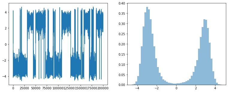
Double well potential#
def double_well(x, k=1, a=3):

    energy = 0.25*k*((x-a)**2) * ((x+a)**2)
    force = -k*x*(x-a)*(x+a)

    return energy, force

@widgets.interact(k=(0.1, 1), a=(0.1,3))
def plot_harm_force(k=1, a=3):

    x = np.linspace(-6,6,1000)

    energy, force = double_well(x, k, a)

    plt.plot(x, energy, '-o',lw=3)
    plt.plot(x, force, '-', lw=3, alpha=0.5)

    plt.ylim(-20,40)
    plt.grid(True)
    plt.legend(['$U(x)$', '$F=-\partial_x U(x)$'], fontsize=15)
# Ininital conditions
x     = 0.1
v     = 0.5

# Input parameters of simulation
kBT   = 5 # vary this
gamma = 0.1 # vary this

dt    = 0.05
t_max = 10000
freq  = 10

times, pos, vel, KE, PE = langevin_md_1d(x, v, dt, kBT, gamma, t_max, double_well)
fig, ax =plt.subplots(nrows=1, ncols=2, figsize=(13,5))

x = np.linspace(min(pos), max(pos), 50)


ax[0].plot(pos)
ax[1].hist(pos, bins=50, density=True, alpha=0.5);

v = np.linspace(min(vel), max(vel),50)
Additional resoruces for learning MD#
For a quick dive consult the following lecture notes:
The best resource for comprehensive stuyd remains the timeless classic by Daan Frankel
Problems#
1D harmonic potential#
Given a 1D potential \(U(x)\) write code to carry out molecular dynamics
Using langevin dynamics to simulate the system in NVT ensemble.
Your input should read in A, B, C parameters, starting point and velocity, timestep and number of iterations, kBT, gamma.
Output should be the positions which should then be histogrammed to obtain probability distribution
Use A=-1, B = 0.0, C = 1.0. Try various initial positions. Look for some interesting regions to sample by adjusting initital positions.
Use A=-1, B = -1, C = 1.0. Again try various initial strting positions.
Beads and springs#
Simulate a chain of harmonic oscillators with the following potential energy function
Take the particle at \(x_0 = 0\) fixed. Carry out constant T MD using langevin dynamics
Try N = 2, N=10 particles and obtain equilibrium distributions of \(x_{j}-x_{j-1}\) for various temperatures.