Entropy and Information

Entropy and Information#

What you will learn

Entropy is a measure of information or uncertainty, quantified using probability distributions.
When expressed in $\log_2$, entropy represents the number of binary (yes/no) questions needed to identify a microstate within a macrostate.
Entropy quantifies the diversity of microstates, reaching its maximum for a uniform (flat) distributions.
The Maximum Entropy (MaxEnt) principle provides the most unbiased way to infer probability distributions given empirical constraints.
In MaxEnt Entropy what we are maximizing is Relative Entropy with respect to reference system where all microstates are equally probable.
Relative entropy quantifies the information lost when approximating one probability distribution with another.
Relative entropy also shows that information (or uncertainty) tends to increase irreversibly in the absence of external interventions.
Relative entropy encodes statistical Distinguishability between forwrad and reverse processes known as the thermodynamic arrow of time.

Surprise#

Which of these two statements conveys the most information?

I will eat some food tomorrow.
I will see a giraffe walking by my apartment.

A measure of information (whatever it may be) is closely related to the element of… surprise!

has very high probability and so conveys little information,
has very low probability and so conveys much information.

If we quanitfy suprise we will quantify information

Addititivity of Information#

Knowledge leads to gaining information

Which is more surprising (contains more information)?

E1: The card is heart? $P(E_1) = \frac{1}{4}$
E2:The card is Queen? $P(E_2) = \frac{4}{52} = \frac{1}{13}$
E3: The card is Queen of hearts? $P(E_1 \, and\, E_2) = \frac{1}{52}$

Knowledge of event should add up our information: $I(E) \geq 0$

We learn the card is heart $I(E_1)$
We learn the card is Queen $I(E_2)$
$I(E_1 and E_2) = I(E_1) + I(E_2)$

A logarithm of probability is a good candidate function for information!

\[log_2 P(E_1) P(E_2) = log_2 P(E_1) + log_2(E_2)\]

What about the sign?

\[I_i = -log_2 p_i\]

Why bit (base two)#

Consider symmetric a 1D random walk with equal jump probabilities. We can view Random walk = string of Yes/No questions.
Imagine driving to a location how many left/right turn informations you need to reach destination?
You gain one bit of information when you are told Yes/No answer

\[I(X=0) = I(X=1) = -log_2 \frac{1}{2} = 1\]

To decode N step random walk trajectory we need N bits.

\[(x_0,x_1,...x_N) = 10111101001010100100\]

Shannon Entropy and Information#

If we want to understand the overall uncertainty in the system, we need to consider all possible outcomes weighted by their probability of occurrence.
This means that rather than looking at the surprise of a single event, we consider the average surprise one would experience over many trials drawn from $p$.
Thus, we take the expectation of surprise over the entire distribution $\langle -log p \rangle$ arriving at a formula known as Shaonon’s expression of Entropy.

Shanon Entropy

\[S = -\sum_i p_i log_2 p_i\]

$S$ Entropy(Information) measured in bits
$p_i$ probability of microstate $i$, e.g coin flip or die roll outcomes

One often uses $H$ to denote Shanon Entropy ($log_2$) and letter $S$ with $log_e$ for entropy in units of Boltzman constant $k_B$
For now lets just roll with $k_B=1$ we wont be doing any thermodynamics in here.
John von Neumann advice to [To Calude Shanon], “You should call it Entropy, for two reasons. In the first place you uncertainty function has been used in statistical mechanics under that name. In the second place, and more importantly, no one knows what entropy really is, so in a debate you will always have the advantage.”

Show code cell source Hide code cell source

import numpy as np
import matplotlib.pyplot as plt

def binary_entropy(p):
    """
    Compute the binary Shannon entropy for a given probability p.
    Avoid issues with log(0) by ensuring p is never 0 or 1.
    """
    return -p * np.log2(p) - (1 - p) * np.log2(1 - p)

# Generate probability values, avoiding the endpoints to prevent log(0)
p_vals = np.linspace(0.001, 0.999, 1000)
H_vals = binary_entropy(p_vals)

# Create a figure with two subplots side-by-side
fig, ax = plt.subplots(1, 2, figsize=(14, 6))

# Plot 1: Binary Shannon Entropy Function
ax[0].plot(p_vals, H_vals, lw=4, color='midnightblue',
           label=r"$H(p)=-p\log_2(p)-(1-p)\log_2(1-p)$")
ax[0].set_xlabel(r"Probability $p$)", fontsize=14)
ax[0].set_ylabel("Entropy (bits)", fontsize=14)
ax[0].set_title("Binary Shannon Entropy",  fontsize=16)
ax[0].legend(fontsize=12)
ax[0].grid(True)

# Plot 2: Example Distributions and Their Entropy
# Define a few example two-outcome distributions:
distributions = {
    "Uniform (0.5, 0.5)": [0.5, 0.5],
    "Skewed (0.8, 0.2)": [0.8, 0.2],
    "Extreme (0.99, 0.01)": [0.99, 0.01]
}

# Colors for each distribution
colors = ["skyblue", "salmon", "lightgreen"]

# For visual separation, use offsets for the bars
width = 0.25
x_ticks = np.arange(2)  # positions for the two outcomes

for i, (label, probs) in enumerate(distributions.items()):
    # Compute the Shannon entropy for the distribution
    entropy_val = -np.sum(np.array(probs) * np.log2(probs))
    # Offset x positions for clarity
    x_positions = x_ticks + i * width - width
    ax[1].bar(x_positions, probs, width=width, color=colors[i],
              label=f"{label}\nEntropy = {entropy_val:.2f} bits")
    
# Set labels and title for the bar plot
ax[1].set_xticks(x_ticks)
ax[1].set_xticklabels(["Outcome 1", "Outcome 2"], fontsize=12)
ax[1].set_ylabel("Probability", fontsize=14)
ax[1].set_title("Example Distributions", fontsize=16)
ax[1].legend(fontsize=12)
ax[1].grid(True, axis='y')

plt.tight_layout()
plt.show()

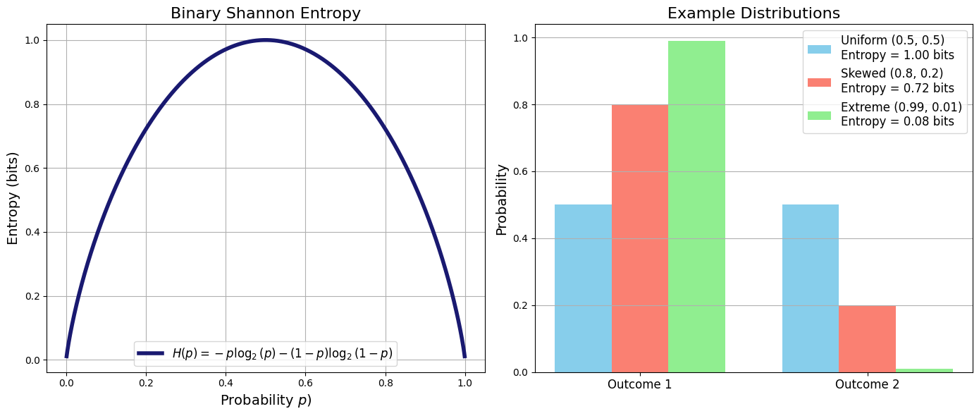
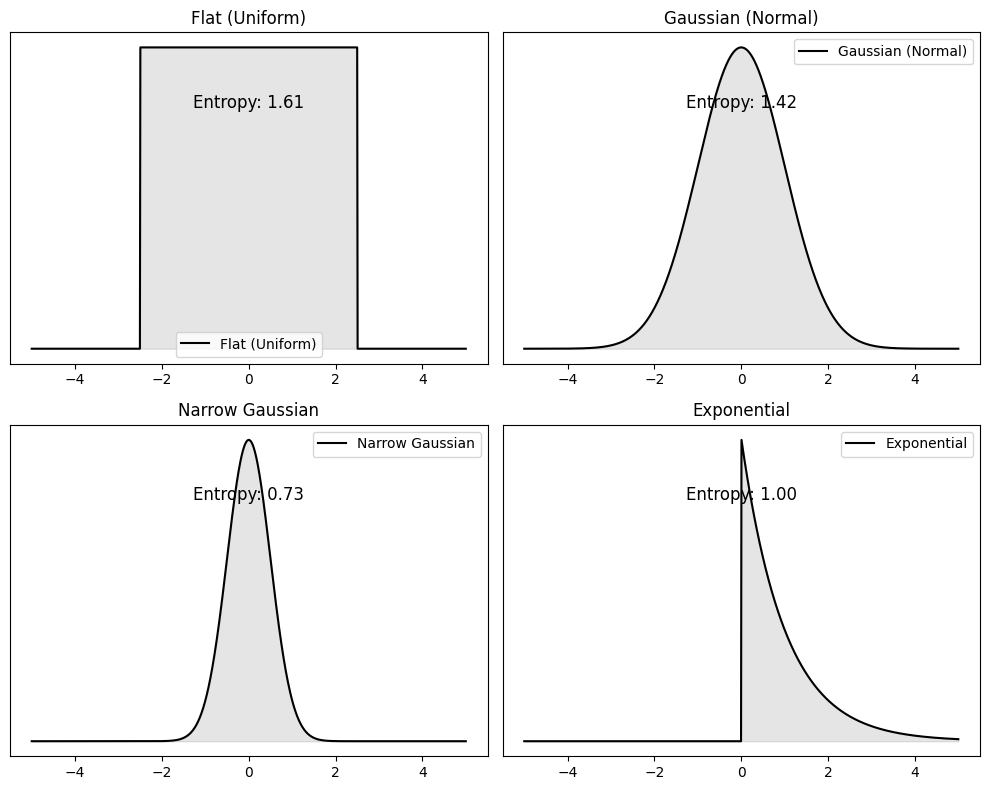
../_images/e7cf3ffc3c37cf204816778fddcb2afbfdf184c7dc4d8f34e2caf39894a622ee.png

To reiterate once again from Shannon formula $S=\sum_i -p_ilogp_i$ we see clearly that Entropy is a statistical quantity characterized by the probability distribution over all possibilities.
The more uncertain (unpredictable) the outcome the higher the entropy of the probability distribution that generates it.

../_images/55251b65d9aee8ab9896c1b7fe5898a25e46e8485a8fa2d6e23bbce818fa1885.png

Exercise: Information per letter $I(m)$ to decode the message

Let $m$ represent the letters in an alphabet. For example:
- Korean: 24 letters
- English: 26 letters
- Russian: 33 letters
The information content associated with these alphabets satisfies:

\[ I(\text{Russian}) > I(\text{English}) > I(\text{Korean}) \]
The information of a sequence of letters is additive, regardless of the order in which they are transmitted:

\[ I(m_1, m_2) = I(m_1) + I(m_2) \]
Question If the symbols of English alphabet (+ blank) appear equally probably, what is the information carried by a single symbol? This must be $log_2(26 + 1) = 4.755$ bits, but for actual English sentences, it is known to be about $1.3$ bits. Why?

Exercise: entropy of die rolls

How much knowledge we need to find out outcome of fair dice?
We are told die shows a digit higher than 2 (3, 4, 5 or 6). How much knowledge does this information carry?

Exercise: Two cats

There are two kittens. We are told that at least one of them is a male. What is the information we get from this message?

Exercise: Monty Hall problem

There are five boxes, of which one contains a prize. A game participant is asked to choose one box. After they choose one of the five boxes, the “coordinator” of the game identifies as empty three of the four unchosen boxes. What is the information of this message?

Exercise: Why are there non-integer number of YES/NO questions??

Explain the origin of the non-integer information. Why it takes less than one-bit to encode information?

Entropy, micro and macro states#

When all $\Omega$ number of microstates of the system have equal probability $p_i=\frac{1}{\Omega}$ the entropy of the system is:

\[S= -\sum \frac{1}{\Omega} log \frac{1}{\Omega} = -\Omega \cdot \frac{1}{\Omega} log \frac{1}{\Omega} = log\Omega\]

We arrive at an expression of Entropy first obtained by Boltzmann where thermal energy units (Boltzman’s) constant were used.

Entropy expression for equally probable microstates

\[S(\Omega) = k_B log \Omega\]

$\Omega$ Number of Microsates availible to the system
$k_B$ Boltzmann’s constant.

Entropy for a macrostate A which has $\Omega(A)$ number of microstates can be written in terms of macrostate probability

\[P(A) = \frac{\Omega(A)}{\Omega}\]

\[S(A) = log \Omega(A) = log P(A) + const\]

Entropy of a macrostate quantifies how probable that macrostate is!. This is yet another manifestation of Large Deviation Theorem we encountered before

\[P(A) \sim e^{S(A)}\]

Flashback to Random Walk, Binomial, and Large Deviation Theorem

Where have we seen the entropy expression before?
When we took the log of the binomial distribution! But why did we call it entropy?

\[ S(n) = \log \frac{N!}{n! (N-n)!} = N \left[ - f \log f - (1-f) \log (1-f) \right] = N s(f) \]

Here, $ f = n/N $ represents the fraction (empirical probability) of steps to the right in a random walk.
$ s(f) = S/N $ is the entropy per particle (or per step), while $ S $ is the total entropy.
Different macrostates have different entropy, depending on the number of microstates they contain!

\[ P(n) = \frac{\Omega(n)}{\Omega_{\text{total}}} = \frac{N!}{n! (N-n)!} \cdot \frac{1}{2^N} \]
where $ \Omega_{\text{total}} = 2^N $ is the total number of microstates.
Once again, we can think of the entropy of a macrostate as being related to its probability:

\[ S(f) \sim \log P(f) \]

Connection to the Large Deviation Theorem
When we express probability in terms of entropy, we recover the Large Deviation Theorem, which states that fluctuations from the most likely macrostates are exponentially suppressed:

\[ P(f) \sim e^{N s(f)} \]

This result highlights how entropy naturally governs the likelihood of macrostates in statistical mechanics.

Interpretations of Entropy#

1. Entropy as a Measure of Information#

Entropy quantifies the amount of information needed to specify the exact microstate of a system.
This can be understood as the number of yes/no (binary) questions required to identify a specific microstate.
Examples:
- Determining the exact trajectory of an $N$-step random walk.
- Identifying the detailed molecular distribution of gas particles in a container.

2. Entropy as a Measure of Uncertainty#

A more uniform (flat) probability distribution of microstates corresponds to higher entropy, whereas a more concentrated (narrow) distribution leads to lower entropy.
Higher entropy implies greater uncertainty about microstates.
- In a high-entropy system, identifying the exact microstate is much harder.
- In contrast, a low-entropy system is more predictable, as fewer microstates are accessible.
When all microstates are equally probable, entropy simplifies to be just the logarithm of the number of microstates, $S = k_B \log \Omega$.
A system will naturally tend to evolve toward macrostates with higher entropy because they correspond to a larger number of available microstates, making them statistically more likely.

3. Physical and Thermodynamic Implications#

Systems with high entropy have a vast number of possible microstates, meaning more “work” is needed—in an informational sense—to pinpoint a specific one.
Reducing entropy requires physical work:
- Example: To reduce the number of yes/no questions needed to specify the position of gas molecules, one must compress the gas, which requires energy.
Spontaneous and irreversible processes tend to increase entropy:
- Entropy naturally increases in isolated systems because evolution toward more probable (higher entropy) macrostates is statistically favored.
- This principle underlies the Second Law of Thermodynamics, which states that entropy never decreases in a closed system.

Is Information Physical?#

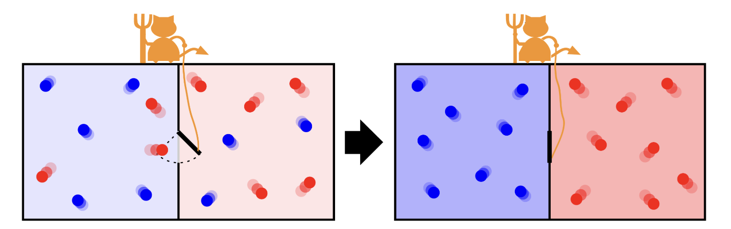
diffflux — Fig. 11 Maxwell’s demon controlling the door that allows the passage of single molecules from one side to the other. The initial hot gas gets hotter at the end of the process while the cold gas gets colder.#

Wheeler’s “It from Bit”:
- Every “it” — every particle, every field, every force, and even the fabric of space-time — derives its function, meaning, and very existence from binary answers to yes-or-no questions. In essence, Wheeler’s idea of “It from Bit” posits that at the most fundamental level, the physical universe is rooted in information. This perspective implies that all aspects of reality are ultimately information-theoretic in origin.
Maxwell’s Demon:
- Maxwell’s Demon is a thought experiment that challenges the second law of thermodynamics by envisioning a tiny being capable of sorting molecules based on their speeds. By selectively allowing faster or slower molecules to pass through a gate, the demon appears to reduce entropy without expending energy. However, the act of gathering and processing information incurs a thermodynamic cost, ensuring that the overall entropy balance is maintained. This paradox underscores that information is a physical quantity with measurable effects on energy and entropy.

Maximum Entropy (MaxEnt) Principle#

Probability represents our incomplete information. Given partial knowledge about some variables how should we construct a probability distribution that is unbiased beyond what we know?
The Maximum Entropy (MaxEnt) Principle provides the best approach: we choose probabilities to maximize Shannon entropy while satisfying given constraints.
This ensures the least biased probability distribution possible, consistent with the available information.

\[ S = - \sum_k p_k \log p_k. \]

We seek to maximize $ S(p) $ subject to the constraints:

\[ \sum_k p_k = 1, \quad \sum_k p_k \, x_k = \langle x \rangle, \quad \sum_k p_k \, y_k = \langle y^b \rangle, \quad \text{etc.} \]

To enforce these constraints, we introduce Lagrange multipliers $ \lambda_0, \lambda_1, \lambda_2, \dots $, leading to the Lagrangian (also called the objective function):

\[ J[p] = - \sum_k p_k \log p_k - \lambda_0 \left( \sum_k p_k - 1 \right) - \lambda_1 \left( \sum_k p_k \, x_k - \langle x \rangle \right) - \lambda_2 \left( \sum_k p_k \, y_k - \langle y \rangle \right) - \dots \]
To maximize $ J[p] $, we take its functional derivative with respect to $ p_k $:

\[ \frac{\delta J}{\delta p_k} = - (1 + \log p_k) - \lambda_0 - \lambda_1 x_k - \lambda_2 y_k - \dots = 0. \]

\[ \log p_k = - 1 - \lambda_0 - \lambda_1 x_k - \lambda_2 y_k - \dots \]

\[ p_k = e^{-1 - \lambda_0} e^{- \lambda_1 x_k} e^{- \lambda_2 y_k} \dots \]

Since $ e^{-1 - \lambda_0} $ is simply a constant normalization factor, we define $Z = e^{1+\lambda_0}$ and arrie at final expression for probability distribution:

\[ p_k = \frac{1}{Z} e^{- \lambda_1 x_k} e^{- \lambda_2 y_k} \dots \]

\[ Z = \sum_k e^{- \lambda_1 x_k- \lambda_2 y_k-...} \]

Interperation of MaxEnt
- The probability distribution takes an exponential form in the constrained variables $ x_k, y_k, \dots $.
- The normalization constant $ Z $ (also called the partition function) ensures that the probabilities sum to 1.
- The Lagrange multipliers $ \lambda_1, \lambda_2, \dots $ encode the specific constraints imposed on the system.
- This result is fundamental in statistical mechanics, where it leads to Boltzmann distributions, and in machine learning, where it underpins maximum entropy models.

MaxEnt: Maximize Entropy Subject to Constraints

Step 1: Construct the Entropy Functional with Constraints on variables $x$, $y$, …

\[ J[p] = - \sum_k p_k \log p_k - \lambda_0 \left( \sum_k p_k - 1 \right) - \lambda_1 \left( \sum_k p_k \, x_k - \langle x \rangle \right) - \lambda_2 \left( \sum_k p_k \, y_k - \langle y \rangle \right) - \dots \]
Step 2: Maximize $J[p] $ by Setting $\delta J[p] = 0 $

\[ p_k = \frac{1}{Z} e^{- \lambda_1 x_k- \lambda_2 y_k...} \]

\[ Z = \sum_k e^{- \lambda_1 x_k- \lambda_2 y_k-...} \]

Step 3: Solve for $\lambda_i $ using the constraints

\[ \sum_k p_k \, x_k= \langle x \rangle, \quad \sum_k p_k \, y_k= \langle y \rangle, \, ... \]

Application MaxEnt: Biased Die Example#

If we are given a fair die MaxENt would predict $p_i=1/6$ as there are no constraints.
But suppose we are given a biased die the average outcome of which is rolling on average a number $ \langle x \rangle = 5.5 $. The entropy function to maximize becomes:

\[ J[p_1, p_2, ..] = - \sum p_i \log p_i - \lambda \left( \sum_i p_i - 1 \right) - B \left( \sum_i p_i x_i - 5.5 \right). \]

Solving the variational equation, we find that the optimal probability distribution follows an exponential form:

\[ p_i = \frac{e^{- B x_i}}{Z}, \]

where $ Z $ is the partition function ensuring normalization:

\[ Z = \sum_{i=1}^{6} e^{- B x_i}. \]

To determine $ B $, we use the constraint $ \langle x \rangle = 5.5 $:

\[ \sum_{i=1}^{6} x_i \frac{e^{- B x_i}}{Z} = 5.5. \]

This equation can be solved numerically for $ B $. In many cases, Newton’s method or other root-finding techniques can be employed to find the exact value of $ B $. This distribution resembles the Boltzmann factor in statistical mechanics, where higher outcomes are exponentially less probable.

Newton’s Method for Optimization

Used to find the root $ B^* $ of $ f(B) = 0 $ via iterative refinement.
Given an initial guess $ B_0 $, we update using:

\[ B_{n+1} = B_n - \frac{f(B_n)}{f'(B_n)} \]

Derivation via Taylor Expansion

Expanding $ f(B) $ around $ B_n $:

\[ f(B) \approx f(B_n) + f'(B_n)(B - B_n) \]

Setting $ f(B) = 0 $:

\[ B = B_n - \frac{f(B_n)}{f'(B_n)} \]

Application to Optimization

For minimization, set $ f(B) = g'(B) $ and apply:

\[ B_{n+1} = B_n - \frac{g'(B_n)}{g''(B_n)} \]

This efficiently finds critical points and is useful in MaxEnt problems.

Optimal B: -1.086963747049358
Optimized probability distribution:
P(1) = 0.0029
P(2) = 0.0086
P(3) = 0.0255
P(4) = 0.0755
P(5) = 0.2238
P(6) = 0.6637

../_images/54bd061c7e3dbcf3b2f9fde71e6f6b5c78866fa80d42791464e9e20686a2ff6b.png

Physical constriants on energy

If the system is in thermal contact with a heat bath at temperature $ T $, energy is allowed to fluctuate. The mean energy $ \langle E \rangle = U $ however should be constant hence we use it as constraint:

\[ J = -\sum_k p_k \log p_k - \lambda \left( \sum_k p_k - 1 \right) - \beta \left( \sum_k p_k E_k - U \right). \]

Solving, we obtain the Boltzmann distribution:

\[ p_k = \frac{e^{-\beta E_k}}{Z}, \]

Relative Entropy#

We mentioned that in MaxEnt derivation we maximized entropy relative to an underlying assumption of equal-probability microstates. We make this idea precise here
Consider example of 1D brownian particle starting at $x_0 = 0$ and diffusing freely. Its probability distribution after time $t$ follows a Gaussian:

\[ p(x, t) = \frac{1}{\sqrt{2\pi \sigma^2}} e^{-\frac{x^2}{4Dt}} \]

The Shannon entropy of this distribution is given by:

\[ S(t) = -\int p(x, t) \log p(x, t) \, dx. \]

Evaluating the integral yields nice compact formulla showing that entropy grows with time as molecule diffuse and sparead all over the container.

\[ S(t) = \frac{1}{2} \log (4\pi e Dt). \]

Problem: Grid Dependence of Shannon Entropy

All is good but if we tried to evaluate the integral we would run into serious problem!
Also how to interpret integral expression in terms of binary yes/no quesionts?
A major issue with Shannon entropy is that it depends on the choice of units. If we refine the grid by choosing a smaller $\Delta x$, the computed entropy does not converge to a well-defined value—it diverges! This makes it unsuitable for studying entropy change in diffusion.
To avoid this issue, one can instead use relative entropy (Kullback-Leibler divergence), which remains well-defined and independent of discretization.

Relative Entropy

\[ D_{\text{KL}}(P || Q) = \sum_x P(x) \ln \frac{P(x)}{Q(x)} \]

\[ D_{\text{KL}}(P || Q) = \int P(x) \ln \frac{P(x)}{Q(x)} \, dx. \]

$Q$ reference probability distribution
$P$ true probability distribution or the one we are using/observing.

The Kullback-Leibler (KL) divergence, or relative entropy, measures how much information is lost when using a reference distribution Q
KL is non-negative and equals zero if and only if $P = Q $ everywhere.
KL divergence is widely used in statistical mechanics, information theory, machine learning and thermodynamics as a measure of information loss when approximating one distribution with another.

Flashback to Random Walk and LDT

We have already encountered relative entropy in the random walk problem!
There, we derived what is known as the Large Deviation Theory (LDT) expression, which shows that fluctuations are concentrated around the minima of $ I(f) $—a function that initially seemed mysterious but proved to be fundamental:

\[ P_N (f) \sim e^{-N I(f)}. \]
Now, we recognize that this function is actually the relative entropy between the empirical and true probability distributions as $ N $ increases:

\[ I(f) = f_+ \log \frac{f_+}{p_+} + f_- \log \frac{f_-}{p_-} = D(f || p) \]

\[ P_N (f) \sim e^{-N D(f || p)} \]
Thus, we see that relative entropy quantifies how unlikely it is to observe an empirical fraction $ f $ deviating from the true probability $ p $. The larger the relative entropy $ D(f || p) $, the less likely it is to observe such a deviation!

Assymetry of KL and irreversibility#

Given two normal distributions:

\[ P(x) = \mathcal{N}(\mu_1, \sigma_1^2), \quad Q(x) = \mathcal{N}(\mu_2, \sigma_2^2), \]

We can compute KL divergence analytically showing that the function is assymteric

\[ D_{\text{KL}}(P || Q) = \ln \frac{\sigma_2}{\sigma_1} + \frac{\sigma_1^2 + (\mu_1 - \mu_2)^2}{2\sigma_2^2} - \frac{1}{2}. \]

KL Divergence between two Gaussians

Derivation of KL Divergence Between Two Gaussians

Given two normal distributions:

\[ P(x) = \mathcal{N}(\mu_1, \sigma_1^2), \quad Q(x) = \mathcal{N}(\mu_2, \sigma_2^2), \]

the Kullback-Leibler (KL) divergence is defined as:

\[ D_{\text{KL}}(P || Q) = \int_{-\infty}^{\infty} p(x) \ln \frac{p(x)}{q(x)} \,dx. \]

Step 1: Write Out the Gaussian PDFs The probability density functions of the two Gaussians are:

\[ P(x) = \frac{1}{\sqrt{2\pi \sigma_1^2}} e^{-\frac{(x - \mu_1)^2}{2\sigma_1^2}}, \]

\[ Q(x) = \frac{1}{\sqrt{2\pi \sigma_2^2}} e^{-\frac{(x - \mu_2)^2}{2\sigma_2^2}}. \]

Taking their ratio:

\[ \frac{P(x)}{Q(x)} = \frac{\sigma_2}{\sigma_1} \exp \left[ \frac{(x - \mu_2)^2}{2\sigma_2^2} - \frac{(x - \mu_1)^2}{2\sigma_1^2} \right]. \]

Taking the natural logarithm:

\[ \ln \frac{P(x)}{Q(x)} = \ln \frac{\sigma_2}{\sigma_1} + \frac{(x - \mu_2)^2}{2\sigma_2^2} - \frac{(x - \mu_1)^2}{2\sigma_1^2}. \]

Step 2: Compute the Expectation $ \mathbb{E}_P[\ln P(x)/Q(x)] $

\[ D_{\text{KL}}(P || Q) = \mathbb{E}_P \left[ \ln \frac{P(x)}{Q(x)} \right] = \int P(x) \ln \frac{P(x)}{Q(x)} \,dx. \]

Since expectation under $ P(x) $ means integrating with $ P(x) $, we evaluate the three terms separately.

First term:
$$ \mathbb{E}_P \left[ \ln \frac{\sigma_2}{\sigma_1} \right] = \ln \frac{\sigma_2}{\sigma_1} $$ since it is a constant.
Second term:
Using the property of a Gaussian expectation $ \mathbb{E}_P [(x - \mu_1)^2] = \sigma_1^2 $,

\[ \mathbb{E}_P \left[ \frac{(x - \mu_1)^2}{2\sigma_1^2} \right] = \frac{1}{2}. \]
Third term:
Expanding $ (x - \mu_2)^2 $,

\[ (x - \mu_2)^2 = (x - \mu_1 + \mu_1 - \mu_2)^2. \]

Taking expectation under $ P(x) $,

\[ \mathbb{E}_P \left[ \frac{(x - \mu_2)^2}{2\sigma_2^2} \right] = \frac{1}{2\sigma_2^2} \left( \sigma_1^2 + (\mu_1 - \mu_2)^2 \right). \]

Step 3: Final KL Divergence Formula

Combining all terms, we get:

\[ D_{\text{KL}}(P || Q) = \ln \frac{\sigma_2}{\sigma_1} + \frac{\sigma_1^2 + (\mu_1 - \mu_2)^2}{2\sigma_2^2} - \frac{1}{2}. \]

Computing KL divergence between two gaussians describing diffusion at times $ t_1 $ and $ t_2 $, where their variances are $ \sigma_1^2 = 2D t_1 $ and $ \sigma_2^2 = 2D t_2 $ results in:

\[ D(p_1 \| p_2) = \frac{1}{2} \left( \frac{t_1}{t_2} - 1 + \log \frac{t_2}{t_1} \right) \]

For a diffusion process, if we compare the forward evolutionof diffusion where variance is spreading over time $t_1=t$ with the hypothetical reversed process where guassian contraints into a peak over time $t_2=T-t$ we can see that:

\[ D_{\text{KL}}(P_{\text{forward}} || P_{\text{backward}}) > 0. \]

This indicates that diffusion is an irreversible process in the absence of external driving forces (since it tends to increase entropy). In contrast, a time-reversed diffusion process (all particles contracting back into the initial state) would violate the second law of thermodynamics.
This statistical distinguishability of time-forward and time-reversed processes is often referred to the “”thermodynamic arrow of time” showing that the forward flow of events is distinguishable from its reverse.

../_images/f43c4280d1a32119078073fd2872abb83914aed0d21a83b6d4b1518069b83d77.png

Relative Entropy in Machine learning#

If $ Q(x) $ assigns very low probability to a region where $ P(x) $ is high, the term $ \log \frac{P(x)}{Q(x)} $ becomes large, strongly penalizing $ Q $ for underestimating $ P $.
If $ Q(x) $ is broader than $ P(x) $, assigning extra probability mass to unlikely regions, this does not significantly affect $ D_{\text{KL}}(P || Q) $, because $ P(x) $ is small in those regions.

This asymmetry explains why KL divergence is not a true distance metric. It penalizes underestimation of true probability mass much more than overestimation, making it particularly useful in machine learning where models are trained to avoid assigning near-zero probabilities to observed data.

<function __main__.plot_gaussians(mu1=0, sigma1=1, mu2=1, sigma2=2)>

Problems#

Problem-1: Compute Entropy for gas partitioning#

A container is divided into two equal halves. It contains 100 non-interacting gas particles that can freely move between the two sides. A macrostate is defined by the fraction of particles in the right half $f$.

Write down an exprssion for entropy S(f)
- Consult the section on Random Walk and Combinatorics formula
Evaluate $ S(f) $ for:
- $ f_L = 0.1 $ (10% left, 90% right)
- $ f_L = 0.25 $ (25% left, 75% right)
- $ f_L = 0.5 $ (50% left, 50% right)
Relate entropy to probability using Large Deviation Theory and answer the following questions:
- Which macrostate is most probable?
- How does entropy influence probability?
- Why are extreme fluctuations (e.g., $ f = 0.1 $) unlikely?

Problem-2#

Below we generate three 2D gaussians $P(x,y)$ with varying degree of correltion betwene $x$ and $y$. Run the code to visualize

import numpy as np
import matplotlib.pyplot as plt

# Define mean values
mu_x, mu_y = 0, 0  # Mean of x and y

# Define standard deviations
sigma_x, sigma_y = 1, 1  # Standard deviation of x and y

# Define different correlation coefficients
correlations = [0.0, 0.5, 0.9]  # Varying degrees of correlation

# Generate and plot 2D Gaussian samples for different correlations
fig, axes = plt.subplots(1, 3, figsize=(15, 5))

for i, rho in enumerate(correlations):
    # Construct covariance matrix
    covariance_matrix = np.array([[sigma_x**2, rho * sigma_x * sigma_y],
                                   [rho * sigma_x * sigma_y, sigma_y**2]])
    
    # Generate samples from the 2D Gaussian distribution
    samples = np.random.multivariate_normal([mu_x, mu_y], covariance_matrix, size=1000)
    
    # Plot scatter of samples
    axes[i].scatter(samples[:, 0], samples[:, 1], alpha=0.5)
    axes[i].set_title(f"2D Gaussian with Correlation ρ = {rho}")
    axes[i].set_xlabel("X")
    axes[i].set_ylabel("Y")

plt.tight_layout()
plt.show()

Compute entropy using probability distributions $P(x,y), P(x|y=0), P(x)$ and $P(y)$
Compute relative entropy $D_{KL}(P(x,y)|| p(x) p(y))$ which is known as Mutual Information. How can you interpret this quantity
You will need these functions. Also check out scipy.stats.entropy

Task	`numpy` Function
Compute histogram for $ P(x, y) $	`numpy.histogram2d`
Compute histogram for $ P(x) $, $ P(y) $	`numpy.histogram`
Normalize histograms to get probabilities	`numpy.sum()`
Compute entropy manually	`numpy.log()`, `numpy.sum()`

Problem-3: Gambling with ten sided die#

Take a ten sided die described by random variable $X =1,2....10$
Experiment shows that after many throughs the average number die shows is $E[x]=5$ with variance $V[X] = 1.5$.
Determine probabilities of ten die sides $p(x)$. You can use the code for six sided die in this notebook. But remember there are now two constraints one on mean and one on variance!

Problem-3 Biased Random walker in 2D#

A random walker moves on a 2D grid, taking steps in one of four possible directions:

Each step occurs with unknown probabilities:

\[ p_{\rightarrow}, p_{\leftarrow}, p_{\uparrow}, p_{\downarrow}\]

which satisfy the normalization condition:

\[ p_{\rightarrow} + p_{\leftarrow} + p_{\uparrow} + p_{\downarrow} = 1. \]

Experimental measurements indicate the expected displacement per step:

\[ \mathbb{E}[x] = p_{\rightarrow} - p_{\leftarrow} = \mu_x = 0.2, \quad \mathbb{E}[y] = p_{\uparrow} - p_{\downarrow} = \mu_y = 0.1. \]

Using the Maximum Entropy (MaxEnt) principle, determine the probabilities $ p^* $ by numerically solving an optimization problem.

You will need scipy.minimize(entropy, initial_guess, bounds=bounds, constraints=constraints, method='SLSQP') to do the minimization. Check the documentation to see how it works

Problem-5: Arrow of time in 2D diffusion#

Simulate 2D diffusion using a Gaussian distribution
- Model diffusion in two dimensions with a probability distribution:
  
  \[ P(x, y, t) = \frac{1}{4\pi D t} \exp\left(-\frac{x^2 + y^2}{4 D t}\right) \]
- Generate samples at different time steps $ t $ using numpy.random.normal with time-dependent variance.
Compute the relative entropy as a function of time $ S_{\text{rel}}(t) $
- Use relative entropy (Kullback-Leibler divergence) to compare the probability distributions at time $ t $ with a reference time $ t_0 = 0.1 $:
  
  \[ D_{\text{KL}}(P(x, y, t) || P(x, y, t_0)) \]
Compare forward and reverse evolution of diffusion
- Compute the relative entropy between forward ($ t \to t + \Delta t $) and reverse ($ t \to t - \Delta t $) diffusion distributions.
- Quantify how diffusion leads to irreversible evolution by evaluating:
  
  \[ D_{\text{KL}}(P_{\text{forward}} || P_{\text{reverse}}) \]
Interpret the results
- How does relative entropy change with time?
- Why is the forward process distinguishable from the reverse process?
- What does this tell us about the arrow of time?

Task	`numpy` Function
Compute histogram for \( P(x, y) \)	`numpy.histogram2d`
Compute histogram for \( P(x) \), \( P(y) \)	`numpy.histogram`
Normalize histograms to get probabilities	`numpy.sum()`
Compute entropy manually	`numpy.log()`, `numpy.sum()`