Langevin Equation for Brownian Motion and Mean Square Displacement (MSD)

The Langevin equation describes the motion of a Brownian particle under the influence of random forces:

\[m \frac{d v}{d t} = - \gamma v + \eta(t)\]

where:

• \(m\) is the mass of the particle,

• \(\gamma\) is the friction coefficient,

• \(v\) is the velocity,

• \(\eta(t)\) is a stochastic force modeled as Gaussian white noise with: (\langle \eta(t) \rangle = 0, \quad \langle \eta(t) \eta(t’) \rangle = 2 D \delta(t - t’)) where $D$ is the noise strength.

In the overdamped limit (high friction, negligible inertia), the Langevin equation simplifies to:

\[\frac{d x}{d t} = - \frac{\gamma}{m} x + \frac{1}{m} \eta(t)\]

Numerical Solution and MSD Calculation

The Euler-Maruyama method can be used to simulate the Langevin equation and compute the mean square displacement (MSD) over time. To ensure accuracy, we compute the MSD using an ensemble average over multiple trajectories:

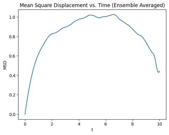
Interpretation of MSD Behavior

• At short times, MSD grows as ballistic motion due to inertia.

• At intermediate times, MSD transitions to diffusive behavior: (\text{MSD}(t) \sim \frac{2 D}{\gamma} (1 - e^{-\gamma t}))

• At long times, noise effects dominate, and MSD saturates due to finite simulation time or numerical artifacts.

By averaging over multiple trajectories, we obtain a more reliable measure of the diffusion process, eliminating artificial decay effects seen in single-trajectory computations.

import numpy as np
import matplotlib.pyplot as plt

def langevin_simulation(num_steps, dt, gamma, D):
    x = np.zeros(num_steps)
    for i in range(1, num_steps):
        noise = np.sqrt(2 * D * dt) * np.random.randn()
        x[i] = x[i-1] - (gamma * x[i-1] * dt) + noise
    return x

def compute_msd_ensemble(num_trajectories, num_steps, dt, gamma, D):
    """Compute the mean square displacement over an ensemble of trajectories."""
    msd = np.zeros(num_steps)
    for _ in range(num_trajectories):
        x_vals = langevin_simulation(num_steps, dt, gamma, D)
        for i in range(num_steps):
            displacements = x_vals[i:] - x_vals[:-i] if i > 0 else np.zeros(num_steps)
            msd[i] += np.mean(displacements**2)
    msd /= num_trajectories
    return msd

# Parameters
num_steps = 1000
dt = 0.01
gamma = 1.0
D = 0.5
num_trajectories = 100

# Compute MSD over an ensemble
msd_vals = compute_msd_ensemble(num_trajectories, num_steps, dt, gamma, D)

# Plot results
plt.plot(np.arange(num_steps) * dt, msd_vals)
plt.xlabel("t")
plt.ylabel("MSD")
plt.title("Mean Square Displacement vs. Time (Ensemble Averaged)")
plt.show()