Statistical mechanics of fluids#
General exprssion of probability distribution of fluids in phase space#
The probability of a state in a classical fluid system is \(f(x^N, p^N)\)
Momentum and position coordinates are separated thanks to the form of kinetic and potential energy terms
Kinetic energy part giveus us Maxwell-Botlzman distribution or the ideal gas part of the partition function \(Z_p\)
Potential energy part gives us configruational parition function \(Z_x\) evaluation of which is non-trivial and mostly can be done via simulaions:
Pressure is related to Free energy as
Volume dependence of partition function is in the integration limits! As volume grows, so does partition function. Therefore p is always positive. We can thus conclude that in equilibrium pressure is always a positive quantity
Reduced configruational distribution functions#
Key fact: The full configurational probability \(P(r^N)\) and the partition function \(Q\) do not factorize due to interparticle interactions. Stronger interactions lead to stronger positional correlations.
Joint probability of particle positions:
To describe the probability of finding particles at positions \(r_1, r_2, \dots, r_N\):
Marginal (reduced) probability density:
Probability of finding particles 1 and 2 at positions \(r_1\) and \(r_2\), regardless of others:
Symmetrized reduced pair distribution:
When particles are indistinguishable, the reduced two-particle distribution becomes:
Radial Distribution Function (RDF)#
For an isotropic fluid, the one-particle probability density is uniform:
For an ideal gas, the two-particle (joint) probability density simplifies as:
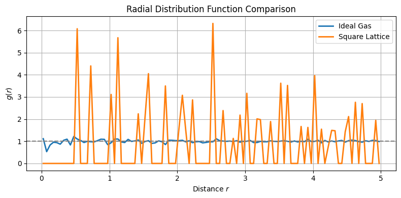
To quantify spatial correlations between particles, we define the Radial Distribution Function (RDF) as:
For an isotropic and homogeneous fluid, RDF depends only on the distance between particles:
Physical meaning of RDF#
Since \(\rho = \rho^{(1)}\), the conditional probability density of finding a particle at distance \(r\) from a tagged particle at the origin is:
Thus, \(\rho g(r)\) represents the average local density at distance \(r\), given a particle is fixed at the origin.
Show code cell source
import numpy as np
import matplotlib.pyplot as plt

# === System parameters ===
N_side = 20                # particles per side for lattice
N = N_side**2              # total particles
L = 10.0                   # box length (L x L)
r_max = L / 2              # max distance for RDF
nbins = 100

# === Make ideal gas configuration ===
positions_ideal = np.random.uniform(0, L, size=(N, 2))

# === Make square lattice configuration ===
spacing = L / N_side
x, y = np.meshgrid(np.linspace(0, L - spacing, N_side),
                   np.linspace(0, L - spacing, N_side))
positions_lattice = np.vstack([x.ravel(), y.ravel()]).T

def compute_rdf(positions, L, r_max, nbins):
    N = len(positions)
    dists = []
    for i in range(N):
        for j in range(i + 1, N):
            dx = positions[i, 0] - positions[j, 0]
            dy = positions[i, 1] - positions[j, 1]

            # Periodic boundary conditions
            dx -= L * np.round(dx / L)
            dy -= L * np.round(dy / L)
            r = np.sqrt(dx**2 + dy**2)
            if r < r_max:
                dists.append(r)

    dists = np.array(dists)
    r_bins = np.linspace(0.0, r_max, nbins + 1)
    r_centers = 0.5 * (r_bins[:-1] + r_bins[1:])
    hist, _ = np.histogram(dists, bins=r_bins)

    dr = r_bins[1] - r_bins[0]
    area = L**2
    rho = N / area
    shell_area = 2 * np.pi * r_centers * dr
    norm = rho * shell_area * (N - 1) / 2  # expected number in each shell
    g_r = hist / norm

    return r_centers, g_r

# === Compute RDFs ===
r_ideal, g_ideal = compute_rdf(positions_ideal, L, r_max, nbins)
r_lattice, g_lattice = compute_rdf(positions_lattice, L, r_max, nbins)

# === Plot ===
plt.figure(figsize=(8, 4))
plt.plot(r_ideal, g_ideal, label='Ideal Gas', lw=2)
plt.plot(r_lattice, g_lattice, label='Square Lattice', lw=2)
plt.axhline(1.0, color='gray', linestyle='--')
plt.xlabel('Distance $r$')
plt.ylabel('$g(r)$')
plt.title('Radial Distribution Function Comparison')
plt.legend()
plt.grid(True)
plt.tight_layout()
plt.show()
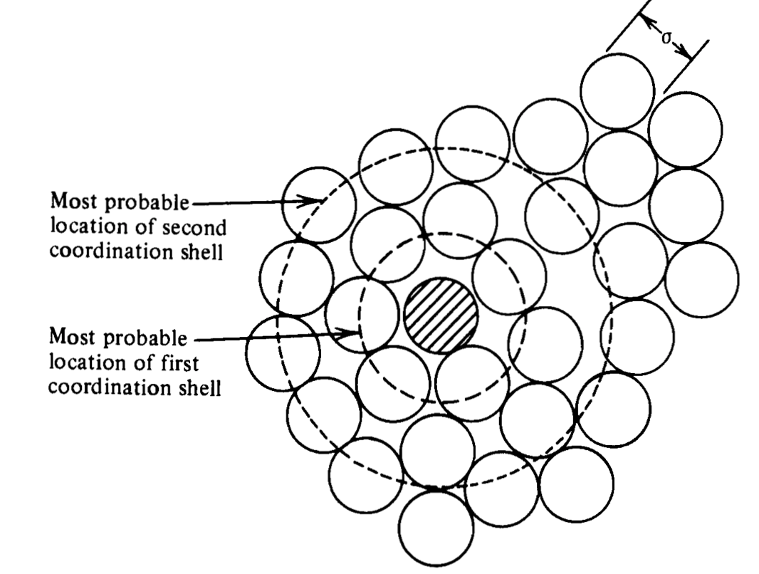
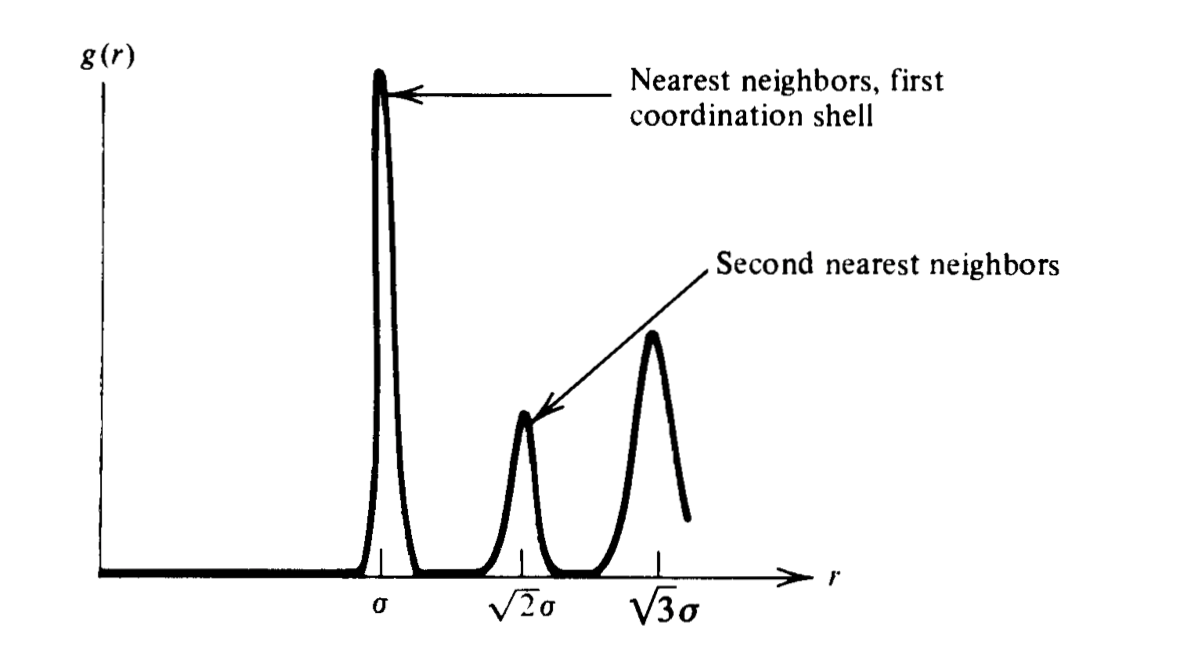
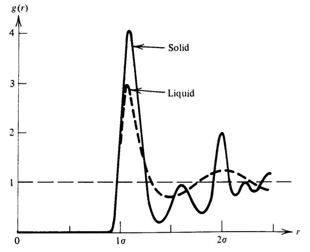
Coordination shells and structure in fluids#

Reversible work theorem and potential of mean force#
Reversible work theorem
\(w(r)\) Reversible work to bring two particles from infinity to distance r
\(g(r)\) Radial distribution function