Molecular Dynamics

Fig. 28 Simulation of Cu atoms

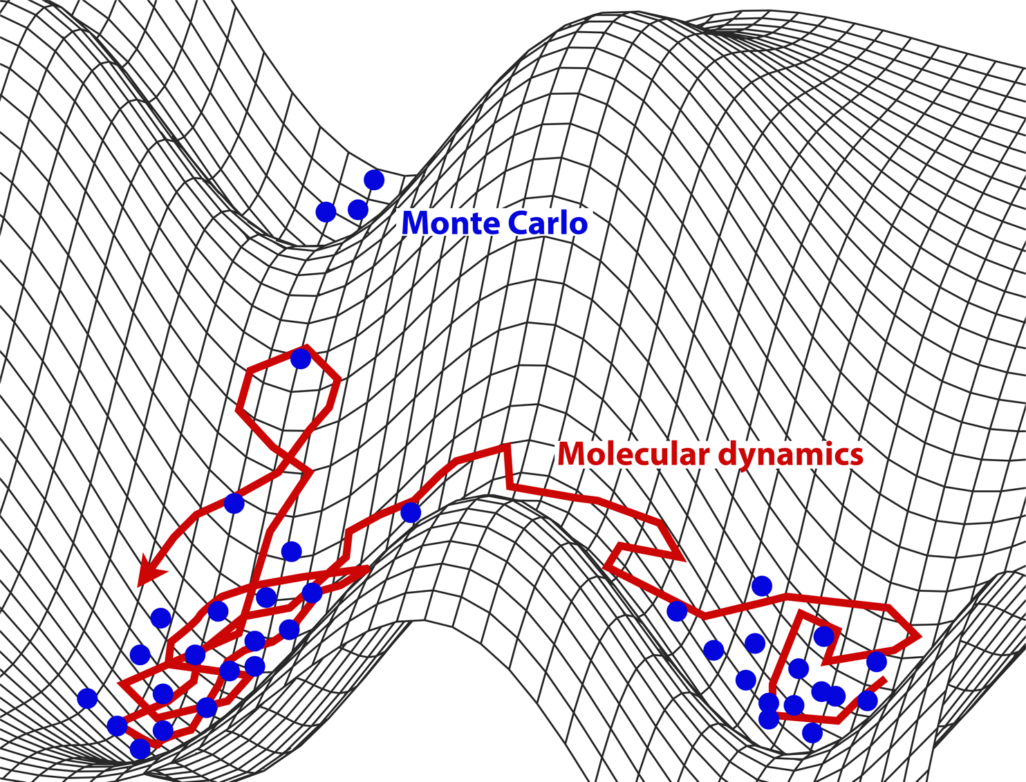
Fig. 29 MD vs MC: Both sample microstates. The former follows the natural motion (dynamics); the latter samples from the Boltzmann distribution using rules designed to improve efficiency.

Timescales and Lengthscales

• Classical Molecular Dynamics can access a hiearrchy of time-scales from pico seconds to microseconds.

• It is also possible to go beyond the time scale of brute force MD byb emplying clever enhanced sampling techniques.

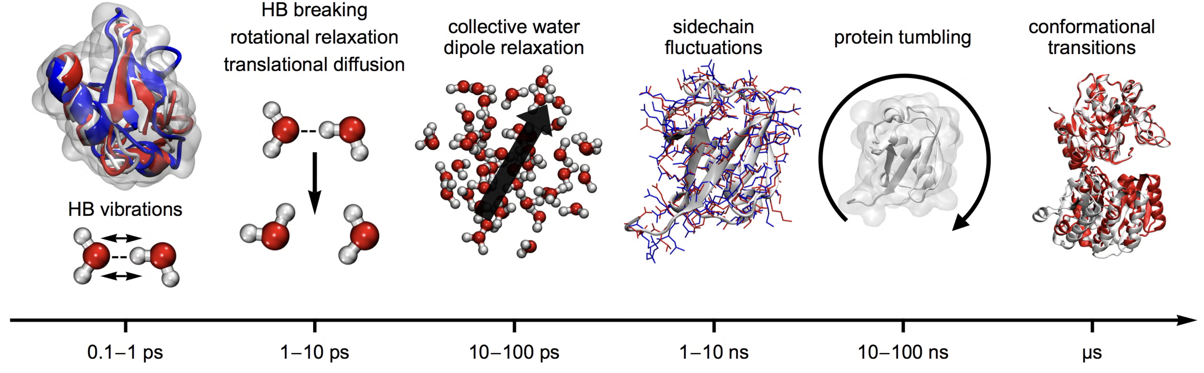
Fig. 30 Different time-scales underlying different leng-scales/motions in molecules

Fig. 31 Simulation of water box

Is MD just Newton’s laws applied on big systems?

Not quite: Noble prize in Chemistry 2013

• Classical molecular dynamics (MD) is a powerful computational technique for studying complex molecular systems.

• Applications span wide range including proteins, polymers, inorganic and organic materials.

• Alos molecular dynamics simulation is being used in a complimentary way to the analysis of experimental data coming from NMR, IR, UV spectroscopies and elastic-scattering techniques, such as small angle scattering or diffraction.

• 2013 Noble Lectures by M Karplus, A Warshell, M Levitt

Integrating equations of motion Numerically

• The Euler method is the simplest numerical integrator for ordinary differential equations (ODEs).

• More accurate integrators that include higher-order terms are known as Runge-Kutta (RK) methods — e.g., RK2, RK4, RK6.

• Given an ODE in standard form:

\[ \frac{d \mathbf{y}}{dt} = \mathbf{f}(t, \mathbf{y}), \]

• we approximate the derivative using finite differences:

\[ \frac{d \mathbf{y}(t)}{dt} \approx \frac{\mathbf{y}_{n+1} - \mathbf{y}_n}{\Delta t}, \]

• leading to the Euler update rule:

\[ \mathbf{y}_{n+1} \approx \mathbf{y}_n + \Delta t \cdot \mathbf{f}(t_n, \mathbf{y}_n). \]

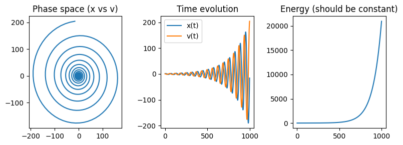
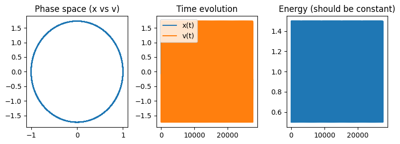
Example: Harmonic Oscillator

The harmonic oscillator with parameters \(m=1, k=1\) is defined by the state vector \(\mathbf{y} = \begin{bmatrix} x \\ v \end{bmatrix}\) with components for \(\dot{y}\) given by:

\[ \dot{x} = v, \quad \dot{v} = -x. \]

\[\begin{split} \frac{d \mathbf{y}}{dt} = \mathbf{f}(\mathbf{y}) = \begin{bmatrix} v \\ -x \end{bmatrix}. \end{split}\]

Using the Euler method, the system evolves as:

\[ \mathbf{y}_{n+1} = \mathbf{y}_n + \Delta t \cdot \mathbf{f}(\mathbf{y}_n). \]

Show code cell source Hide code cell source

import numpy as np
import matplotlib.pyplot as plt

y  = np.array([1.0, 1.0])  # Initial [x, v]
pos, vel = [], []
t  = 0
dt = 0.1 

for i in range(1000):
    
    dydt = np.array([y[1], -y[0]])  # [v, -x]
    y += dt * dydt                  # Euler update
    
    t += dt
    
    pos.append(y[0])
    vel.append(y[1])

# Convert to arrays
pos, vel = np.array(pos), np.array(vel)

# Plot results
fig, ax = plt.subplots(ncols=3, nrows=1, figsize=(8,3))

# Phase space
ax[0].plot(pos, vel)
ax[0].set_title("Phase space (x vs v)")

# Time series
ax[1].plot(pos, label="x(t)")
ax[1].plot(vel, label="v(t)")
ax[1].legend()
ax[1].set_title("Time evolution")

# Energy
ax[2].plot(0.5*pos**2 + 0.5*vel**2)
ax[2].set_title("Energy (should be constant)")

plt.tight_layout()
plt.show()

Verlet algortihm

Taylor expansion of position \(\vec{r}(t)\) after timestep \(\Delta t\) we obtain forward and backward Euler schems

\[r_{t+\Delta t} = r_t +v_t\Delta t +\frac{1}{2}a_t \Delta t^2 + O(\Delta t^3)\]

\[r_{t-\Delta t} = r_t -v_t \Delta t +\frac{1}{2}a_t \Delta t^2 + O(\Delta t^3)\]

• In 1967 Loup Verlet introduced a new algorithm into molecular dynamics simulations which preserves energy is accurate and efficient.

• Summing the two taylor expansion above we get a updating scheme which is an order of mangnitude more accurate

\[r_{t+\Delta t} = 2r_t - r_{t-\Delta t} +a_t \Delta t^2+O(\Delta t^4)\]

\[v_t = \frac{r_{t+\Delta t}-r_{t-\Delta t}}{2\Delta t} +O(\Delta t^2) \]

• Velocity is not needed to update the positions. But we still need them to set the temperature.

• Terms of order \(O(\Delta t^3)\) cancel in position giving position an accuracy of order \(O(\Delta t^4)\)

• To update the position we need positions in the past at two different time points! This is is not very efficient.

Velocity Verlet updating scheme

• A better updating scheme has been proposed known as Velocity-Verlet (VV) which stores positions, velocities and accelerations at the same time. Time stepping backward expansion \(r(t-\Delta t + \Delta t)\) and summing with the forward Tayloer expansions we get Velocity Verlet updating scheme:

\[v_{t+\Delta t} = v_t + \frac{1}{2}(a_t+a_{t+\Delta t})\Delta t +O(\Delta t^3)\]

• Substituting forces \(a=\frac{F}{m}\) instead of acelration we get

\[r_{t+\Delta t} = r_t + v_t\Delta t + \frac{F_t}{2m}\Delta t^2\]

\[v_{t+\Delta t} = v_t + \frac{F_t+F_{t+\Delta t}}{2m}\Delta t\]

Velocity Verlet Algorithm

1. Evaluate the initial force from the current position:

\[ F_t = -\frac{\partial U(r)}{\partial r} \Bigg|_{r(t)} \]

2. Update the position:

\[ r_{t+\Delta t} = r_t + v_t \Delta t + \frac{F_t}{2m} \Delta t^2 \]

3. Partially update the velocity:

\[ v_{t+\Delta t/2} = v_t + \frac{F_t}{2m} \Delta t \]

4. Evaluate the force at the new position:

\[ F_{t+\Delta t} = -\frac{\partial U(r)}{\partial r} \Bigg|_{r(t+\Delta t)} \]

5. Complete the velocity update:

\[ v_{t+\Delta t} = v_{t+\Delta t/2} + \frac{F_{t+\Delta t}}{2m} \Delta t \]

Molecular Dynamics of Classical Harmonic Oscillator (NVE)

Velocity Verlet integration of harmonic oscillator

Show code cell source Hide code cell source

import numpy as np

def run_md_nve_1d(x, v, dt, t_max, en_force):
    """
    Minimalistic 1D Molecular Dynamics simulation (NVE ensemble) 
    using Velocity Verlet integration.
    Simulates a particle moving in a 1D potential without thermal noise or friction
    (i.e., energy-conserving dynamics).
    
    Parameters
    ----------
    x : float
        Initial position.
    v : float
        Initial velocity.
    dt : float
        Time step for integration.
    t_max : float
        Total simulation time.
    en_force : callable
        Function that takes position `x` as input and returns a tuple (potential energy, force).
    
    Returns
    -------
    pos : ndarray
        Array of particle positions over time.
    vel : ndarray
        Array of particle velocities over time.
    KE : ndarray
        Array of kinetic energies over time.
    PE : ndarray
        Array of potential energies over time.
    
    Example
    -------
    >>> def harmonic_force(x):
    >>>     k = 1.0
    >>>     return 0.5 * k * x**2, -k * x
    >>> pos, vel, KE, PE = run_md_nve_1d(1.0, 0.0, 0.01, 10.0, harmonic_force)
    """
    
    times, pos, vel, KE, PE = [], [], [], [], []
    
    # Initialize force and potential energy
    pe, F = en_force(x)
    
    t = 0.0
    for step in range(int(t_max / dt)):
        
        # Velocity Verlet Integration
        
        # Half-step velocity update
        v += 0.5 * F * dt
        
        # Full-step position update
        x += v * dt
        
        # Update force at new position
        pe, F = en_force(x)
        
        # Half-step velocity update
        v += 0.5 * F * dt
        
        # Save results
        times.append(t)
        pos.append(x)
        vel.append(v)
        KE.append(0.5 * v * v)
        PE.append(pe)
        
        # Advance time
        t += dt
    
    return np.array(pos), np.array(vel), np.array(KE), np.array(PE)

Run NVE simulation of harmonic oscillator

Show code cell source Hide code cell source

#----parameters of simulation----
k     = 3 
x0    = 1 
v0    = 0
dt    = 0.01 * 2*np.pi/np.sqrt(k) #A good timestep determined by using oscillator frequency
t_max = 1000

### Define Potential Energy function
def ho_en_force(x, k=k):
    '''Force field of harmonic oscillator:
    returns potential energy and force'''
    
    return k*x**2, -k*x

### Run simulation
pos, vel, KE, PE = run_md_nve_1d(x0, v0, dt, t_max, ho_en_force)

# Plot results
fig, ax = plt.subplots(ncols=3, nrows=1, figsize=(8,3))

# Phase space
ax[0].plot(pos, vel)
ax[0].set_title("Phase space (x vs v)")

# Time series
ax[1].plot(pos, label="x(t)")
ax[1].plot(vel, label="v(t)")
ax[1].legend()
ax[1].set_title("Time evolution")

# Energy
ax[2].plot(0.5*pos**2 + 0.5*vel**2)
ax[2].set_title("Energy (should be constant)")

plt.tight_layout()
plt.show()

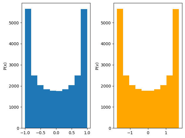
Plot Distribution in phase-space

Show code cell source Hide code cell source

### Visualize
fig, ax =plt.subplots(ncols=2)

ax[0].hist(pos);
ax[1].hist(vel, color='orange');
ax[0].set_ylabel('P(x)')
ax[1].set_ylabel('P(v)')

fig.tight_layout()

Ensemble averages

Ergodic hypothesis

\[\langle A \rangle = \frac{1}{t} \int^{ \tau_{eq} +t}_{ \tau_{eq} } A(t)\]

• \(\tau_{eq}\) time it teks for system to “settle into” equilibrium and \(t\) time of simulation.

• Time averages are equal to ensemble averages when \(t\lim \infty\). But in real life we need to determine how long to sample.

• Ergodic assumption is: during the coruse of MD we visit all the microstates (or small but representative subset) that go into the ensemble average!

Energy conservation in simulations

• Kinetic, potential and total energies are flcutuation quantities in the Molecualr dynamics simulations.

• Energy in (NVE) or its average \(\langle E \rangle\) (in NVT, NPT, etc) must remain constant!

\[KE_t = \sum_i \frac{p_t^2}{2m}\]

\[PE_t = \sum_{ij}u_{ij}(r_t)\]

\[\langle E \rangle = \langle KE \rangle +\langle PE \rangle \approx const \]

Temperature control in simulations

According to equipariting result of equilibrium statistical mechanics in the NVT ensmeble

\[\Big\langle \sum_i \frac{p_t^2}{2m} \Big\rangle =\frac{3 }{2}N k_B T\]

\[T_t = \frac{2}{3 N k_B} \big\langle KE \big\rangle_t \]

Pressure control in simulations

\[P = \frac{1}{3V} \sum^N_i \Big [\frac{p^2_i}{m} +\vec{F}_i(r) \cdot \vec{r}_i(t) \Big ]\]

Langevin equation

• A particle of mass \(m\) moves under the force derived from a potential energy \(U(x)\). The motion is purely deterministic.

\[ m \ddot{x} = -\nabla_x U \]

• Challenge: What should we do when we have only a one or few particles, and cannot explicitly simulate the vast surrounding environment in order to assign temperature?

• Solution: We model the surrounding medium (e.g., a solvent) as an implicit thermal bath that interacts with the particle.

  • The particle exchanges energy with the bath, maintaining thermal equilibrium at a fixed temperature \(T\).

  • This motivates Langevin dynamics, where the effects of the solvent are captured by friction (dissipation) and random thermal kicks (fluctuations), without simulating solvent molecules explicitly.

Langevin Equation

\[ m \ddot{x} = -\nabla_x U - \gamma \dot{x} + \eta(t) \]

Overdamped Limit of Langevin Dynamics (\(m \ddot{x} = 0\))

\[ \gamma \dot{x} = \nabla_x U + \eta(t) \]

• The friction \(\gamma\) and thermal noise \(\eta(t)\) are clearly connected becasue the faster the particle movies (more noise) the more it also dissipates energy.

• the connection is known by the name of Fluctuation-Dissipation Theorem:

Fluctuation-Dissipation Theorem (FDT)

\[ \langle \eta(t) \eta(t') \rangle = 2 \gamma k_B T \, \delta(t - t') \]

• The environment “forgets” what happened almost immediately after a collision very short memory hence noise terms are uncorrelated (independent). Just like what we had in brownian motion.

• The FDT ensures that the strength of random thermal kicks is precisely tuned to the amount of viscous damping, so that the system reaches and maintains thermal equilibrium at temperature \(T\)

• FDT connects diffusion (random spreading) and viscosity (resistance to motion), both fundamentally controlled by temperature.

Derivation of FDT

We consider the underdamped Langevin equation for a free particle (\( U(x) = 0 \)):

\[ m \dot{v}(t) = -\gamma v(t) + \eta(t) \]

Here:

• \( v(t) \) is the velocity,

• \( \gamma \) is the friction coefficient,

• \( \eta(t) \) is Gaussian white noise with:

\[ \langle \eta(t) \eta(t') \rangle = C \delta(t - t') \]

We want to compute the steady-state value of \( \langle v^2(t) \rangle \) and relate it to \( C \), \( \gamma \), and \( T \).

Step 1: Solve the Langevin Equation

We write the equation in standard ODE form:

\[ \dot{v}(t) + \frac{\gamma}{m} v(t) = \frac{1}{m} \eta(t) \]

This is a linear inhomogeneous ODE, solvable by integrating factor:

\[ v(t) = v(0) e^{-\gamma t / m} + \frac{1}{m} \int_0^t e^{-\gamma (t - s) / m} \eta(s) \, ds \]

Step 2: Compute \( \langle v^2(t) \rangle \)

We take the expectation:

\[ \langle v^2(t) \rangle = \left\langle \left[ v(0) e^{-\gamma t / m} + \frac{1}{m} \int_0^t e^{-\gamma (t - s)/m} \eta(s) \, ds \right]^2 \right\rangle \]

This expands to:

\[ \langle v^2(t) \rangle = v^2(0) e^{-2\gamma t / m} + \frac{2 v(0) e^{-\gamma t / m}}{m} \left\langle \int_0^t e^{-\gamma (t - s)/m} \eta(s) \, ds \right\rangle + \frac{1}{m^2} \left\langle \left( \int_0^t e^{-\gamma (t - s)/m} \eta(s) \, ds \right)^2 \right\rangle \]

• The second term is zero since \( \langle \eta(s) \rangle = 0 \),

• For the third term, use the noise correlation:

\[ \left\langle \left( \int_0^t e^{-\gamma (t - s)/m} \eta(s) \, ds \right)^2 \right\rangle = \int_0^t \int_0^t e^{-\gamma (2t - s - s')/m} \langle \eta(s) \eta(s') \rangle \, ds \, ds' = C \int_0^t e^{-2\gamma (t - s)/m} \, ds \]

Change variable: \( u = t - s \Rightarrow du = -ds \)

\[ = C \int_0^t e^{-2\gamma (t - s)/m} \, ds = C \int_0^t e^{-2\gamma u/m} \, du = \frac{C m}{2\gamma} \left( 1 - e^{-2\gamma t/m} \right) \]

So the full result is:

\[ \langle v^2(t) \rangle = v^2(0) e^{-2\gamma t/m} + \frac{C}{2 m \gamma} \left( 1 - e^{-2\gamma t/m} \right) \]

Long-Time Limit

As \( t \to \infty \), the exponential terms vanish:

\[ \boxed{ \langle v^2 \rangle = \lim_{t \to \infty} \langle v^2(t) \rangle = \frac{C}{2 m \gamma} } \]

Apply Equipartition

At thermal equilibrium, equipartition gives:

\[ \left\langle \frac{1}{2} m v^2 \right\rangle = \frac{1}{2} k_B T \quad \Rightarrow \quad \langle v^2 \rangle = \frac{k_B T}{m} \]

Matching with the derived expression:

\[ \frac{C}{2 m \gamma} = \frac{k_B T}{m} \quad \Rightarrow \quad C = 2 \gamma k_B T \]

\[ \boxed{ \langle \eta(t) \eta(t') \rangle = 2 \gamma k_B T \, \delta(t-t') } \]

Molecualr Dynamics of Harmonic oscillator (NVT)

• Our goal is to Numerically solve the Langevin equation:

\[ m \ddot{x} = -\nabla V(x) - \gamma \dot{x} + \sqrt{2\gamma k_BT} \, \eta(t), \]

• The target is to sample the canonical distribution:

\[ P(x, v) \propto \exp\left( -\beta \left( \frac{1}{2} m v^2 + V(x) \right) \right). \]

• There are many ways of simulating langevin. Simplest is to use Euler method just like we did for diffusion.

• Here we will use BAOAB scheme which splits the Langevin evolution operator into three pieces:

  • B: Free drift in position (\(x\) evolution under \(v\)).

  • A: Velocity change under conservative force \(F = -\nabla V(x)\).

  • O: Stochastic process (friction + random kicks in \(v\)).

• Thus, BAOAB updates position and velocity via a B → A → O → A → B sequence at each timestep \(\Delta t\).

Feature	Explanation
Stability	Handles both large and small friction \(\gamma\) robustly
Accuracy	Samples correct Boltzmann distribution up to \(\mathcal{O}(\Delta t^2)\) errors
Efficiency	Large stable timesteps allowed compared to naive Euler schemes
Universality	Reduces to velocity Verlet (Hamiltonian MD) if \(\gamma=0\) and to overdamped Langevin if \(\gamma \to \infty\)

BAOAB scheme

1. B: Drift half-step in position

   \[ x \to x + \frac{\Delta t}{2} v \]

2. A: Kick velocity half-step using force

   \[ v \to v + \frac{\Delta t}{2m} F(x) \]

3. O: Apply stochastic friction and noise to velocity

   \[ v \to e^{-\gamma \Delta t} v + \sqrt{k_B T (1 - e^{-2\gamma \Delta t})/m} \, R, \]

   where \(R\) is a standard normal random number.

4. A: Kick velocity half-step again

   \[ v \to v + \frac{\Delta t}{2m} F(x) \]

5. B: Drift half-step in position

   \[ x \to x + \frac{\Delta t}{2} v \]

Show code cell source Hide code cell source

def langevin_md_1d(x, v, dt, kBT, gamma, t_max, en_force):
    '''Langevin dynamics applied to 1D potentials
    Using integration scheme known as BA-O-AB.
    INPUT: Any 1D function with its parameters
    '''
    
    times, pos, vel, KE, PE  = [], [], [], [], []
    
    t = 0  
    for step in range(int(t_max/dt)):
        
        #B-step
        pe, F = en_force(x)
        v    += F*dt/2
        
        #A-step
        x += v*dt/2

        #O-step
        v = v*np.exp(-gamma*dt) + np.sqrt(1-np.exp(-2*gamma*dt)) * np.sqrt(kBT) * np.random.normal()
        
        #A-step
        x +=  v*dt/2
        
        #B-step
        pe, F = en_force(x)
        v    +=  F*dt/2
        
        ### Save output 
        times.append(t), pos.append(x), vel.append(v), KE.append(0.5*v*v), PE.append(pe)    
    
    return np.array(times), np.array(pos), np.array(vel), np.array(KE), np.array(PE)
     

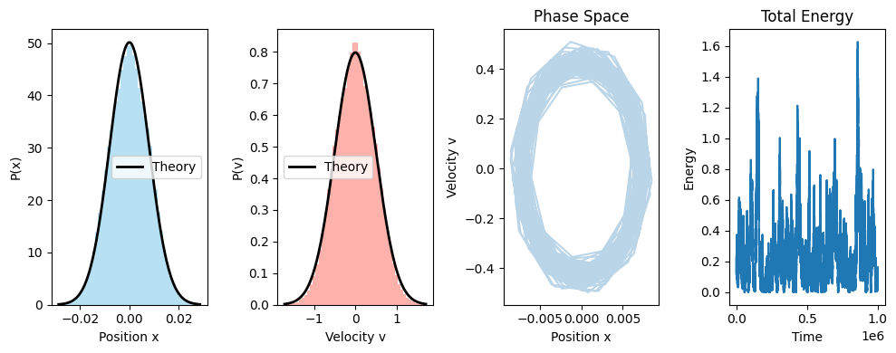
Run lagevin dynamics of 1d harmonic oscillator

Show code cell source Hide code cell source

import numpy as np
import matplotlib.pyplot as plt

# Initial conditions
x0 = 0.0
v0 = 0.5

# Input parameters
kBT   = 0.25
gamma = 0.01
dt    = 0.01
t_max = 10000
freq  = 10
k     = (2 * np.pi * freq)**2  # Spring constant (harmonic oscillator)

### Define Potential: Energy and Force
def ho_en_force(x, k=k):
    energy = 0.5 * k * x**2
    force  = -k * x
    return energy, force

### Langevin dynamics (assuming you have this function correctly defined)
# Should return arrays: times, pos, vel, KE, PE
times, pos, vel, KE, PE = langevin_md_1d(x0, v0, dt, kBT, gamma, t_max, ho_en_force)

### Plotting
fig, ax = plt.subplots(nrows=1, ncols=4, figsize=(10, 4))

bins = 50

# Theoretical distributions
def gaussian_x(x, k, kBT):
    return np.exp(-k*x**2/(2*kBT)) / np.sqrt(2*np.pi*kBT/k)

def gaussian_v(v, kBT):
    return np.exp(-v**2/(2*kBT)) / np.sqrt(2*np.pi*kBT)

# Plot histograms
ax[0].hist(pos, bins=bins, density=True, alpha=0.6, color='skyblue')
ax[1].hist(vel, bins=bins, density=True, alpha=0.6, color='salmon')

# Plot theoretical curves
x_grid = np.linspace(min(pos), max(pos), 300)
v_grid = np.linspace(min(vel), max(vel), 300)

ax[0].plot(x_grid, gaussian_x(x_grid, k, kBT), 'k-', lw=2, label='Theory')
ax[0].set_xlabel('Position x')
ax[0].set_ylabel('P(x)')
ax[0].legend()


ax[1].plot(v_grid, gaussian_v(v_grid, kBT), 'k-', lw=2, label='Theory')
ax[1].set_xlabel('Velocity v')
ax[1].set_ylabel('P(v)')
ax[1].legend()

ax[2].plot(pos[-1000:], vel[-1000:], alpha=0.3)
ax[2].set_xlabel('Position x')
ax[2].set_ylabel('Velocity v')
ax[2].set_title('Phase Space')

E_tot=KE+PE
ax[3].plot(E_tot)
ax[3].set_xlabel('Time')
ax[3].set_ylabel('Energy')
ax[3].set_title('Total Energy')

fig.tight_layout()
plt.show()

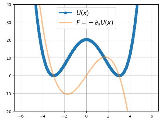
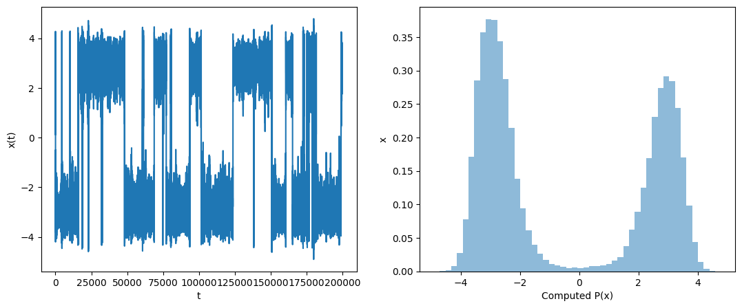
Double well potential

Show code cell source Hide code cell source

def double_well(x, k=1, a=3):
    
    energy = 0.25*k*((x-a)**2) * ((x+a)**2)
    force = -k*x*(x-a)*(x+a)
    
    return energy, force
 
x = np.linspace(-6,6,1000)
energy, force = double_well(x) 

plt.plot(x, energy, '-o',lw=3)
plt.plot(x, force, '-', lw=3, alpha=0.5)

plt.ylim(-20,40)
plt.grid(True)
plt.legend(['$U(x)$', '$F=-\partial_x U(x)$'], fontsize=15)

<matplotlib.legend.Legend at 0x7f3eb43922b0>

Show code cell source Hide code cell source

# Potential 
def double_well(x, k=1, a=3):
    
    energy = 0.25*k*((x-a)**2) * ((x+a)**2)
    force = -k*x*(x-a)*(x+a)
    
    return energy, force

# Ininital conditions
x     = 0.1
v     = 0.5

# Input parameters of simulation
kBT   = 5 # vary this
gamma = 0.1 # vary this
dt    = 0.05
t_max = 10000
freq  = 10

#### Run the simulation
times, pos, vel, KE, PE = langevin_md_1d(x, v, dt, kBT, gamma, t_max, double_well)

#### Plotting 
fig, ax =plt.subplots(nrows=1, ncols=2, figsize=(13,5))

x = np.linspace(min(pos), max(pos), 50)

ax[0].plot(pos)
ax[1].hist(pos, bins=50, density=True, alpha=0.5);

v = np.linspace(min(vel), max(vel),50)

ax[0].set_xlabel('t')
ax[0].set_ylabel('x(t)')

ax[1].set_xlabel('Computed P(x)')
ax[1].set_ylabel('x')

Text(0, 0.5, 'x')

Additional resoruces for learning MD

• Goran Wahnstrom’s MD and MC lectures

• Online course materials: principles of modern molecular simulation methods

• “Understanding Molecular Simulation: From Algorithms to Applications” a book by Daan Frankel

Problems

1D potential

• In molecular simulations, we often want to sample from the Boltzmann distribution \(P(x) \propto e^{-V(x)/k_BT}\).

• Langevin dynamics enables us to do this by modeling the effects of both deterministic forces (from the potential) and random thermal fluctuations.

• Write a Python function using NumPy to simulate a 1D system under Langevin dynamics for the following potential:

\[ V(x) = Ax^2 + Bx^3 + Cx^4 \]

You should:

1. Implement Langevin dynamics to evolve position and velocity over time.

2. Allow inputs for:

   • Coefficients A, B, C

   • Initial position and velocity

   • Time step dt, number of steps

   • Temperature kBT and friction coefficient gamma

3. Store all positions and plot a normalized histogram (probability density) after the simulation.

4. Try the following setups:

   • Double well: A = -1, B = 0, C = 1

   • Asymmetric well: A = -1, B = -1, C = 1

   • Vary initial positions and explain what changes

5. Compare your histograms with \(e^{-V(x)/k_BT}\). Do they match?

6. What happens if gamma is very small? What about very large?