MD/MC simulations of fluids#
What you will learn
Molecular dynamics: Solve Newton’s equations of motion for many particles.
Velocity Verlet algorithm: A symplectic, time-reversible integration method.
Periodic boundary conditions: Simulate a small part of a bulk system.
Minimum image convention: Correct distance calculation across periodic boundaries.
Lennard-Jones fluid: Standard model for simple liquids.
Temperature control: Via velocity rescaling.
Structural analysis: Computation of the radial distribution function \(g(r)\).
Molecular Dynamics Simulation of a Lennard-Jones Fluid#
The code in this notebook simulates a collection of particles interacting through the Lennard-Jones (LJ) potential using Molecular Dynamics (MD) in 3D.
The simulation is designed to be efficient, modular, and easy to understand, leveraging NumPy and object-oriented programming (OOP).Particles are initially arranged in a face-centered cubic (FCC) lattice and evolved over time using the Velocity Verlet algorithm under periodic boundary conditions.
The simulation tracks: Kinetic Energy (KE), Potential Energy (PE), Pressure, Pair correlation function \(g(r)\)
Physical Model of LJ fluid#
Each particle experiences a force given by the Lennard-Jones potential:
\(r\) is the distance between two particles.
The potential is cut off at a radius (r_c) to improve efficiency.
The system is simulated at a fixed temperature by rescaling velocities during the early steps (velocity rescaling).
PBC#
If a particle leaves the box, it re-enters at the opposite side.
What should be the distance between partiles? There is some mbiguity because distance between atoms may now include crossing the system boundary and re-entering. This is identical to introducing copies of the particles around the simulation box. We adopt minimum image convention by choosing the shortest distance possible
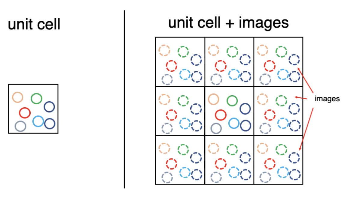
Fig. 32 Perioidc Boundary Conditions#
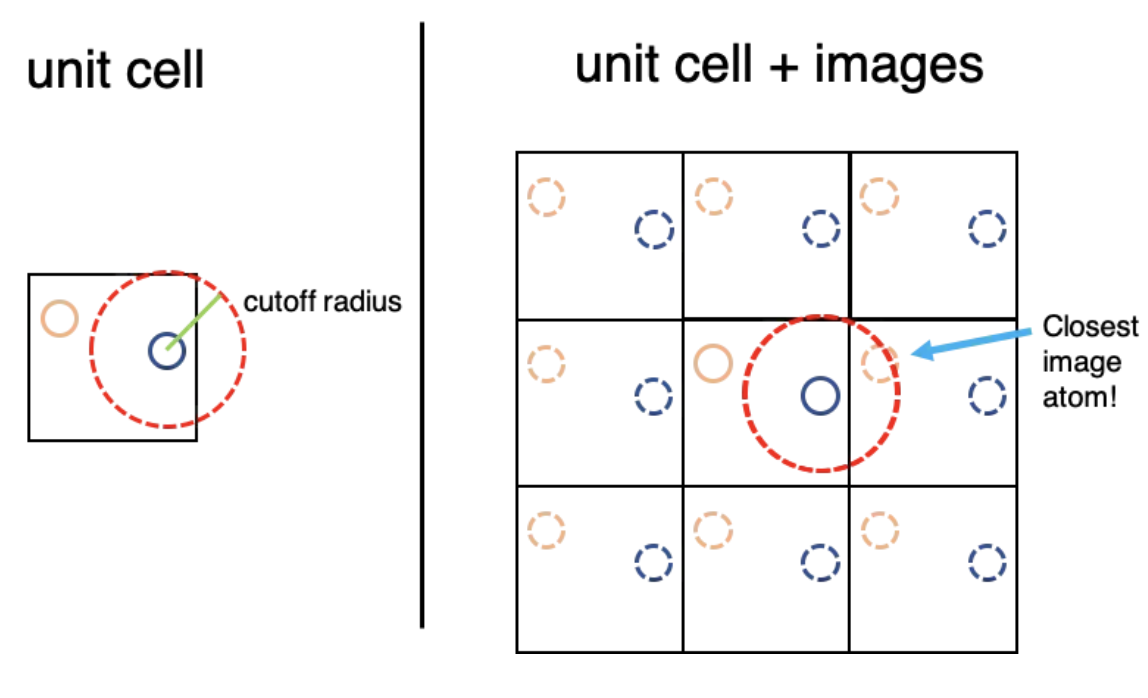
Fig. 33 Minimum Image Convention showing that we only track particles with clsoest distance.#
MD of LJ fluid#
Velocity Verlet Algorithm
1. Evaluate the initial force from the current position:
2. Update the position:
3. Partially update the velocity:
4. Evaluate the force at the new position:
5. Complete the velocity update:
Show code cell source
import numpy as np
import matplotlib.pyplot as plt

class LJSystem:
    def __init__(self, rho=0.88, N_cell=3, T=1.0, rcut=2.5):
        # System parameters
        self.N = 4 * N_cell**3
        self.rho = rho
        self.L = (self.N / rho)**(1/3)
        self.T_target = T
        self.rcut = rcut
        self.rcut_sq = rcut**2

        # Create FCC lattice positions
        base = np.array([[0, 0, 0], [0.5, 0.5, 0], [0.5, 0, 0.5], [0, 0.5, 0.5]])
        pos = np.array([b + [i, j, k] for i in range(N_cell) for j in range(N_cell) for k in range(N_cell) for b in base])
        self.pos = pos * (self.L / N_cell)

        # Velocities
        self.vel = np.random.randn(self.N, 3)
        self.vel -= np.mean(self.vel, axis=0)

        # Indices for upper triangular part
        self.I, self.J = np.triu_indices(self.N, k=1)

    def minimum_image(self, r_vec):
        return (r_vec + self.L/2) % self.L - self.L/2

    def compute_forces(self):
        r_vec = self.minimum_image(self.pos[self.I] - self.pos[self.J])
        r_sq = np.sum(r_vec**2, axis=1)

        mask = r_sq < self.rcut_sq
        r_vec = r_vec[mask]
        r_sq = r_sq[mask]

        r2_inv = 1.0 / r_sq
        r6_inv = r2_inv**3

        dU_dr = 48 * r6_inv * (r6_inv - 0.5) * r2_inv
        F_ij = dU_dr[:, None] * r_vec

        # Forces on each particle
        forces = np.zeros_like(self.pos)
        np.add.at(forces, self.I[mask],  F_ij)
        np.add.at(forces, self.J[mask], -F_ij)

        # Potential energy
        U = 4 * np.sum(r6_inv * (r6_inv - 1))

        # Virial for pressure
        Pvir = np.sum(np.sum(F_ij * r_vec, axis=1))

        # Histogram for g(r)
        hist, _ = np.histogram(np.sqrt(r_sq), bins=30, range=(0, self.L/2))

        return forces, U, Pvir, hist

    def integrate(self, dt):
        forces, U, Pvir, hist = self.compute_forces()
        self.vel += 0.5 * dt * forces
        self.pos = (self.pos + dt * self.vel) % self.L
        forces_new, U_new, Pvir_new, hist_new = self.compute_forces()
        self.vel += 0.5 * dt * forces_new
        kin = 0.5 * np.sum(self.vel**2)
        return kin, U_new, Pvir_new, hist_new

    def rescale_velocities(self, kin):
        """Velocity rescaling to maintain target temperature"""
        factor = np.sqrt(3 * self.N * self.T_target / (2 * kin))
        self.vel *= factor

    def simulate(self, dt=0.005, nsteps=5000, freq_out=50):
        kins, pots, Ps, hists = [], [], [], []
        for step in range(nsteps):
            kin, pot, Pvir, hist = self.integrate(dt)

            if step < 1000:  # Temperature stabilization
                self.rescale_velocities(kin)

            if step % freq_out == 0:
                kins.append(kin)
                pots.append(pot)
                Ps.append(Pvir)
                hists.append(hist)

        return np.array(kins), np.array(pots), np.array(Ps), np.mean(hists, axis=0)
Example simulation and analysis#
# Initialize system
lj = LJSystem(rho=0.88, N_cell=3, T=1.0)

# Run simulation
kins, pots, Ps, hist = lj.simulate(dt=0.005, nsteps=10000, freq_out=50)

# Post-processing
r = np.linspace(0, lj.L/2, 30)
dr = r[1] - r[0]
shell_volumes = 4*np.pi*r**2*dr
g_r = hist / (lj.N * lj.rho * shell_volumes)

# Plot
plt.plot(r, g_r, '-o')
plt.xlabel(r'$r$')
plt.ylabel(r'$g(r)$')
plt.show()
---------------------------------------------------------------------------
KeyboardInterrupt                         Traceback (most recent call last)
Cell In[2], line 5
      2 lj = LJSystem(rho=0.88, N_cell=3, T=1.0)
      4 # Run simulation
----> 5 kins, pots, Ps, hist = lj.simulate(dt=0.005, nsteps=10000, freq_out=50)
      7 # Post-processing
      8 r = np.linspace(0, lj.L/2, 30)

Cell In[1], line 76, in LJSystem.simulate(self, dt, nsteps, freq_out)
     74 kins, pots, Ps, hists = [], [], [], []
     75 for step in range(nsteps):
---> 76     kin, pot, Pvir, hist = self.integrate(dt)
     78     if step < 1000:  # Temperature stabilization
     79         self.rescale_velocities(kin)

Cell In[1], line 63, in LJSystem.integrate(self, dt)
     61 self.vel += 0.5 * dt * forces
     62 self.pos = (self.pos + dt * self.vel) % self.L
---> 63 forces_new, U_new, Pvir_new, hist_new = self.compute_forces()
     64 self.vel += 0.5 * dt * forces_new
     65 kin = 0.5 * np.sum(self.vel**2)

Cell In[1], line 34, in LJSystem.compute_forces(self)
     31 r_sq = np.sum(r_vec**2, axis=1)
     33 mask = r_sq < self.rcut_sq
---> 34 r_vec = r_vec[mask]
     35 r_sq = r_sq[mask]
     37 r2_inv = 1.0 / r_sq

KeyboardInterrupt:
MC simulation#
MCMC of LJ fluid
Randomly pick a particle.
Propose a random displacement.
Compute the change in energy \(\Delta E\).
Accept or reject the move based on the Metropolis criterion:
If the move is rejected, the particle returns to its previous position.
Show code cell source
import numpy as np
import matplotlib.pyplot as plt

class LJ_MC_System:
    def __init__(self, rho=0.88, N_cell=3, T=1.0, rcut=2.5):
        # System parameters
        self.N = 4 * N_cell**3
        self.rho = rho
        self.L = (self.N / rho)**(1/3)
        self.T = T
        self.beta = 1.0 / T
        self.rcut = rcut
        self.rcut_sq = rcut**2

        # Create FCC lattice positions
        base = np.array([[0, 0, 0], [0.5, 0.5, 0], [0.5, 0, 0.5], [0, 0.5, 0.5]])
        pos = np.array([b + [i, j, k] for i in range(N_cell) for j in range(N_cell) for k in range(N_cell) for b in base])
        self.pos = pos * (self.L / N_cell)

        # Pair indices
        self.I, self.J = np.triu_indices(self.N, k=1)

    def minimum_image(self, r_vec):
        return (r_vec + self.L/2) % self.L - self.L/2

    def total_energy(self):
        r_vec = self.minimum_image(self.pos[self.I] - self.pos[self.J])
        r_sq = np.sum(r_vec**2, axis=1)
        mask = r_sq < self.rcut_sq
        r2_inv = 1.0 / r_sq[mask]
        r6_inv = r2_inv**3
        return 4 * np.sum(r6_inv * (r6_inv - 1))

    def particle_energy(self, idx):
        rij = self.minimum_image(self.pos[idx] - self.pos)
        r_sq = np.sum(rij**2, axis=1)
        mask = (r_sq < self.rcut_sq) & (r_sq > 0)  # exclude self-interaction
        r2_inv = 1.0 / r_sq[mask]
        r6_inv = r2_inv**3
        return 4 * np.sum(r6_inv * (r6_inv - 1))

    def mc_move(self, max_disp=0.1):
        idx = np.random.randint(self.N)
        old_pos = self.pos[idx].copy()
        old_energy = self.particle_energy(idx)

        # Propose move
        displacement = (np.random.rand(3) - 0.5) * 2 * max_disp
        self.pos[idx] = (self.pos[idx] + displacement) % self.L

        new_energy = self.particle_energy(idx)
        dE = new_energy - old_energy

        # Metropolis criterion
        if np.random.rand() > np.exp(-self.beta * dE):
            # Reject move
            self.pos[idx] = old_pos

    def sample(self):
        """ Sample pair distances for g(r) """
        r_vec = self.minimum_image(self.pos[self.I] - self.pos[self.J])
        r_sq = np.sum(r_vec**2, axis=1)
        hist, _ = np.histogram(np.sqrt(r_sq), bins=30, range=(0, self.L/2))
        return hist

    def simulate(self, nsteps=50000, freq_out=500):
        hists = []
        energies = []

        for step in range(nsteps):
            self.mc_move()

            if step % freq_out == 0:
                hist = self.sample()
                hists.append(hist)
                energies.append(self.total_energy())

        return np.array(energies), np.mean(hists, axis=0)
Example MC simulation and analysis#
# ----------------- Main -----------------

# Initialize system
lj_mc = LJ_MC_System(rho=0.88, N_cell=3, T=1.0)

# Run simulation
energies, hist = lj_mc.simulate(nsteps=100000, freq_out=500)

# Post-processing
r = np.linspace(0, lj_mc.L/2, 30)
dr = r[1] - r[0]
shell_volumes = 4*np.pi*r**2*dr
g_r = hist / (lj_mc.N * lj_mc.rho * shell_volumes)

# Plot
plt.plot(r, g_r, '-o')
plt.xlabel(r'$r$')
plt.ylabel(r'$g(r)$')
plt.show()
Differences of Monte Carlo vs Molecular Dynamics#
Monte Carlo (MC) |
Molecular Dynamics (MD) |
|---|---|
No real dynamics, just configurations |
Real-time evolution of particle trajectories |
Samples equilibrium ensemble directly |
Samples via time evolution |
No conservation laws |
Energy/momentum conserved after equilibration |
Easier to implement |
More complex (forces, integration needed) |
Faster for static properties like \(g(r)\) |
Necessary for dynamics (diffusion, viscosity) |
Problems#
MD sim of LJ fluid#
Modify the cut-off radius \(r_c\) and observe its effect on pressure and energy.
Remove velocity rescaling after equilibration and check energy conservation.
Implement a thermostat (e.g., Andersen, Berendsen) instead of manual rescaling.
Compute the diffusion coefficient from particle trajectories.
Visualize the particle trajectories over time (animation!).
MC sim of LJ fluid#
Vary sim parameters
Tune maximum displacement (
max_disp) to optimize acceptance rate (~40%-50% is ideal).Check how \(g(r)\) changes when density or temperature changes.
Implement energy cutoffs with shifted potentials to smooth out the energy at \(r_c\).
Try simulating hard spheres (infinite repulsion at contact).
Phases of LJ fluid#
Run MD or MC simulations of LJ fluid at several temperatures to identify critical temperature.
At each temperature evaluate heat capacity and RDFs.
Plot how energy, heat capacity and RDF change as a function of temperature.
Study dependence on sampling efficiency on magnitude of particle displacement.