Phase transitions: a birds eye view#
Phases, Phase diagrams and Phase-transitions#
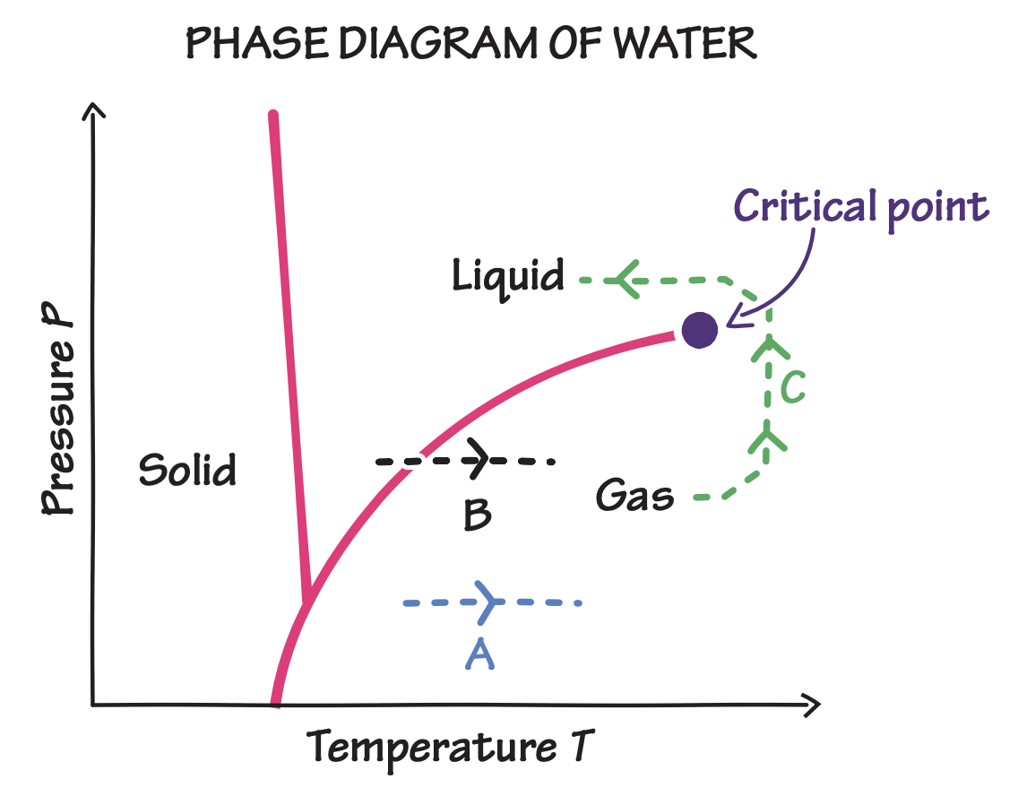
Fig. 22 Phaase-diagram for fluids. The path A does not lead to change of phase. The Path B leads to abrupt phase-transition. Path C side-steps phase boundary and hence there is no abrupt change!#
History of phase transitions#
1895 Pierre Curie in his doctoral thesis studies types of magnetism, discovers
The effect of temperature
A phase transition happening at the Curie point
The phenomenon occurs at the atomic scale

1920 – Lenz introduces a lattice model for ferromagnetism#
Lenz argued that “atoms are dipoles which turn over between two positions.”
In a quantum-theoretical treatment, these dipoles would largely occupy two distinct orientations.
1920 – Lenz suggests a project to his PhD student, who develops a 1D spin lattice model#
Each site on the lattice represents a spin state, either +1 or –1.
Only nearest-neighbor interactions are considered.
The model is simple, but foundational.
1924 – Ernst Ising’s PhD thesis: No phase transition!?
Ising finds no phase transition in the one-dimensional model.
He dismisses the model as overly simplistic and mathematical.
Incorrectly concludes that no phase transition occurs in any dimension.
Leaves academic research to teach college-level physics.
Despite its flaws, the paper draws attention from major figures (Pauli, Heisenberg, Dirac), who agree it’s too simplified.
1936 – Rudolf Peierls: Surprising proof of phase transition in 2D
Peierls proves that in two dimensions, the Lenz-Ising model does undergo a finite-temperature phase transition.
His result revitalizes interest in the model and shows the importance of dimensionality.
1941 – Kramers and Wannier calculate the critical temperature
Develop a method to estimate the critical temperature for the 2D Ising model.
Predict self-duality in the system, paving the way for exact solutions.
1944 – Onsager solves the 2D Ising model analytically
A landmark achievement in theoretical physics.
Exact expressions derived for partition function, magnetization, and other thermodynamic quantities.
Lars Onsager, trained as a chemist, made significant contributions; other chemists like Ben Widom followed suit in developing phase transition theory.
1944– Ising model becomes a canonical system for studying phase transitions
Following Onsager’s work, the model becomes central in mathematical physics.
Studied with various mathematical techniques: transfer matrix, cluster expansion, combinatorics, and more.
Applications broaden to biology, chemistry, economics, and computer science.
1970s – Renormalization Group (RG) theory developed by Kenneth Wilson (Nobel Prize, 1982)
The Curie critical point is shown to be universal, exhibiting translation, scale, and rotation invariance.
Introduces powerful concepts: renormalization, scale invariance, universality, and coarse-graining.
RG revolutionizes our understanding of critical phenomena.
1985 – Conformal Field Theory (CFT)
Provides an elegant framework to describe critical systems in two dimensions.
Explains universality classes via symmetry principles.
Links statistical mechanics and quantum field theory in a deep and fruitful way.
Becomes a cornerstone in modern theoretical physics.
Ising models: The H atom of phase transitions#
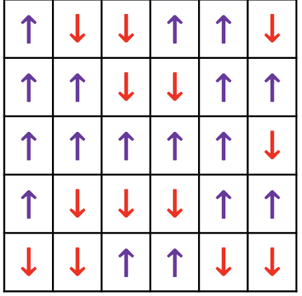
Fig. 23 Ising model is defined on a lattice where eaach site can be occupied with one spin having up or down orientation.#
1st order vs 2nd order phjase transition#
.png)
Fig. 24 First and second order transitons#
Critical Phenomena: Correlation length diverges#
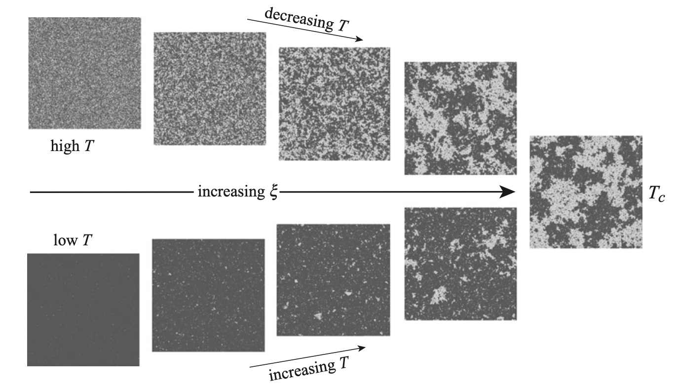
Fig. 25 Critical Phenomena showing divergence of correlations#
Critical Phenomena: Universaility at critical points#
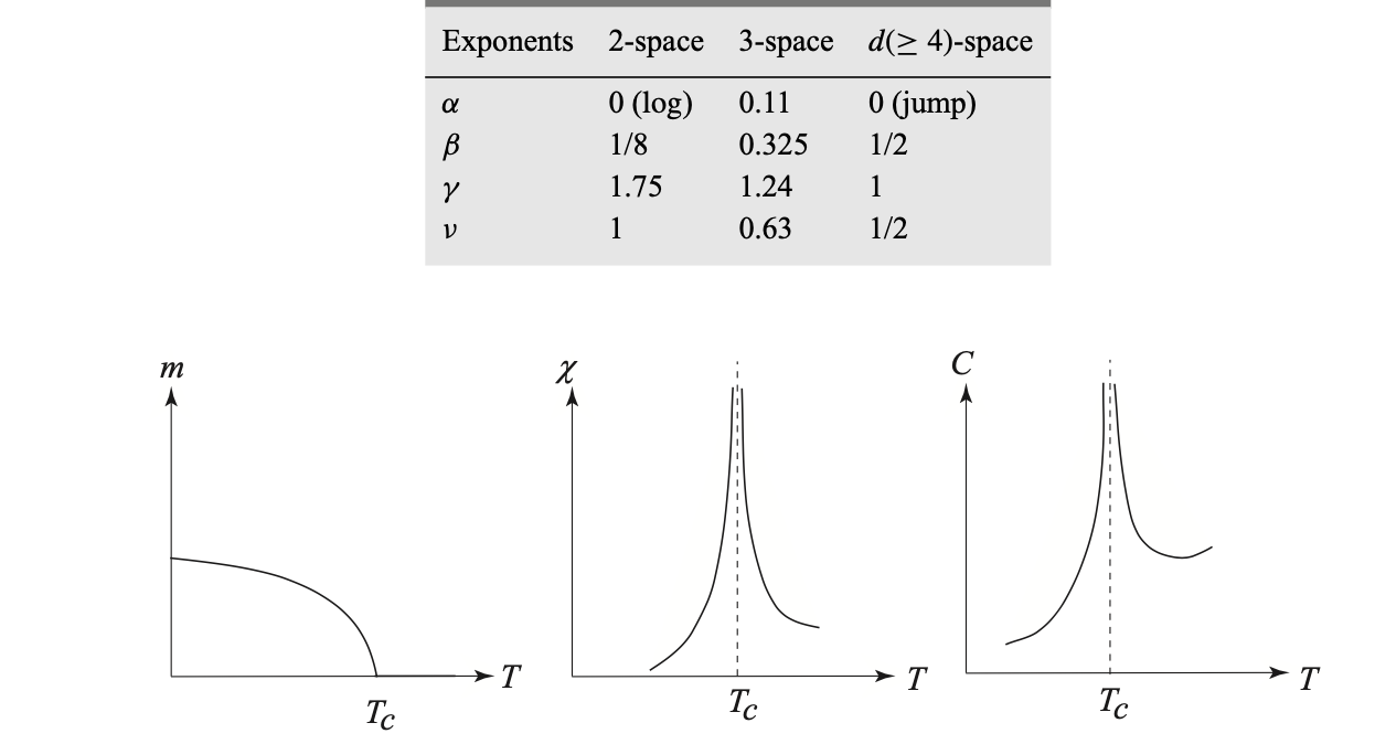

Universality#
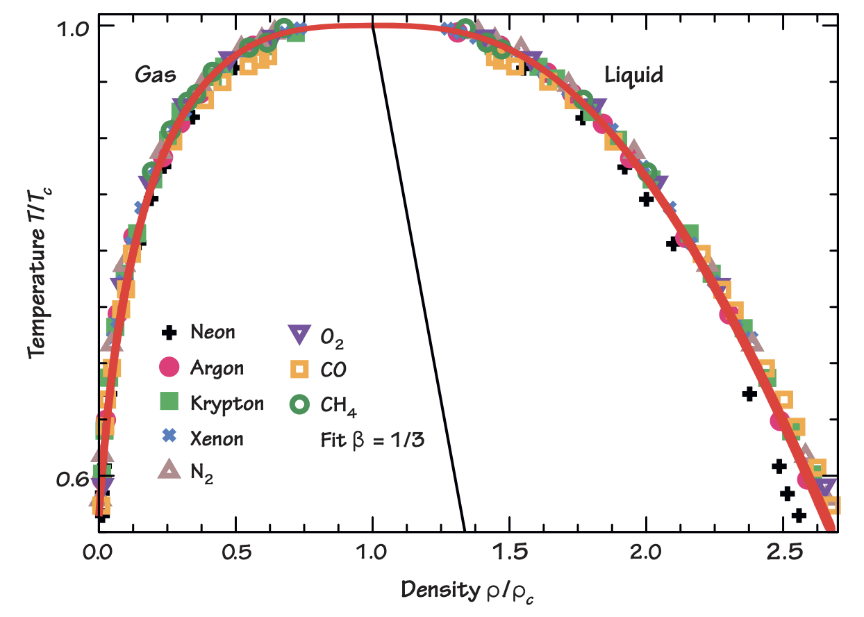
Fig. 26 Universality illustrated on phase-diagram of fluids#
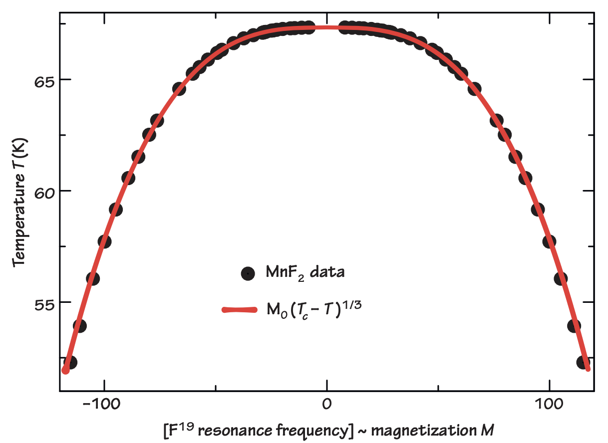
Fig. 27 Universality illustrated on phase-diagram of fluids#
Thermodynamics of magnetic systems#
For magnetic systems placed under external field \(B\) the change in internal energy consists of an extra term of work done by the external field to displace mangetization \(M\)
A free energy as a function of intensive variables can be written down following legendre transform:
Magnetization and Entropy can now be linked to derivatives of free energy
Fluctuations, correlations and susceptibilities#
Heat capacity \(C_v\)
Heat capacity is again the familiar expression established in our treatment of canonical ensemble.
Susceptibility \(\chi\)
Magnetic susceptibility quantifies response of the ssytem to the variation of magnetic field.
Correlation function \(c(i,j)\) and correlation length
At high temperatures, spins on an ising lattice point up and down randomly. While at low temperatures, all spins tend to align. To quantify the degree of alignment, we can define a quantity named correlation length \(\xi\), which can be defined mathematically through correlation function \(c(i,j)\)
Some notable applications of Ising models.#
Ferromagnetism The Ising model is the scalar version of the three-dimensional ‘Heisenberg model’ :
Binary alloys and lattice gases Each lattice site is occupied either by an atom A or B. Nearest neighbour interac- tions are \(\epsilon_{AA}\), \(\epsilon_{BB}\) and \(\epsilon_{AB}\). We identify \(A\) with \(s_i = 1\) and B with \(S_i = −1\). The Hamiltonian then is: \(H = − ∑ J_{ij}s_is_j \langle i,j\rangle\) with \(J_{ij} = \epsilon_{AB} − 0.5(\epsilon_{AA} + \epsilon_{BB})\). Thus the Ising model describes order-disorder transitions in regard to composition.
Spin glasses now each bond is assigned an individual coupling constant J and they are drawn from a random distribution. E.g. one can mix ferromagnetic and anti-ferromagnetic couplings. This is an example for a structurally disordered system, on top of which we can have a thermal order-disorder transition.
Conformations in biomolecules a famous example is the helix-coil transition from biophysics. \(s_i\) a hydrogen bond in a DNA-molecules is closed; \(s_i\) = −1 the bond is open. The phase tran- sition is between a straight DNA-molecule (helix) and a coiled DNA-molecule. Other examples are the oxygen-binding sites in hemoglobin, chemotactic recep- tors in the receptor fields of bacteria, or the molecules building the bacterial flag- ellum, which undergos a conformational switch if the flagellum is rotated in the other direction (switch from run to tumble phases).
Neural networks representing the brain \(s_i = 1\) a synapse is firing, \(s_i = −1\) it is resting. The Hopfield model for neu- ral networks is a dynamic version of the Ising model and Boltzmann machines recognise handwriting by using the Ising model.
Spread of opinions or diseases Spread of opinions, rumours or diseases in a society; these kinds of models are used in socioeconomic physics. If nearest neighbour coupling is sufficiently strong, the system gets ‘infected’.
The Peierls argument for presence/absence of phase transitions in 1D, 2D and 3D#
Starting around 1933, Peierls published scaling arguments why a phase transition should occur in 2D as opposed to 1D
No phase transition in 1D at T>0#
1D case Start with 1D chain of all spin up configuration and create an isalnd of oposite spins.
Energy cost is:
Entropy cost is:
Free Energy differnece:
Thus free energy for \(N\gg1\) is always negative for any finite temperature. It is always favorable to create grain boundaries due to entropic reasons.
Phase transition in 1D cannot occur at finite temperature!
Phase transition in 2D at \(T>0\) realizable#
In 2D and 3D introducing isalnd of spins creates a surface spins sproportional to linear size of the island L which is now a macroscopic quantitiy comparable to N
Energy cost is:
Entropy cost using a crude estimate of random walk on cubic lattice is:
Free Energy differnece: