Ising model#

Microstates of Ising model#

import matplotlib.pyplot as plt
import numpy as np

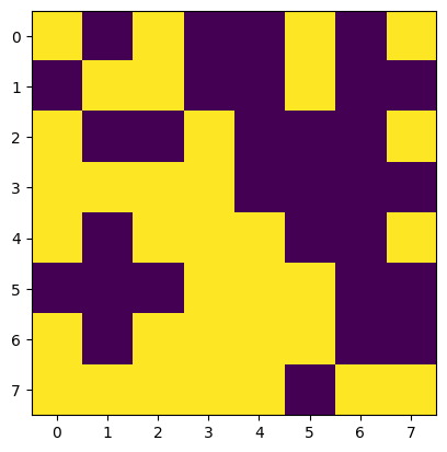
spins = np.random.choice([-1,1],size=(8,8)) # every time you sammple a new microstate

print(spins)

plt.imshow(spins)

[[-1  1 -1 -1 -1  1  1 -1]
 [ 1 -1 -1  1  1 -1 -1  1]
 [ 1  1 -1 -1  1 -1 -1  1]
 [-1 -1 -1  1  1 -1  1 -1]
 [-1 -1 -1  1  1 -1  1  1]
 [ 1  1  1  1 -1 -1  1  1]
 [ 1 -1 -1  1 -1  1  1 -1]
 [ 1 -1  1 -1 -1 -1 -1 -1]]

<matplotlib.image.AxesImage at 0x7f3dc407abe0>

Sampling microstates of Ising Model#

• Monte Carlo appraoch to computing observables is simple: all we have to do is sample from the exponential distribution.

• Problems with regular MC

  • There is an astronomical number of states, $i=1...N^2$!

  • Most of these microstates make exponentially small contribution to probability distribution! $P(E_i)$

  • Brute force MC will not be efficient for sampling important portions of $P(E_i)$.

Extracting thermodynamics from Ising models#

Enforcing periodic boundary conditions#

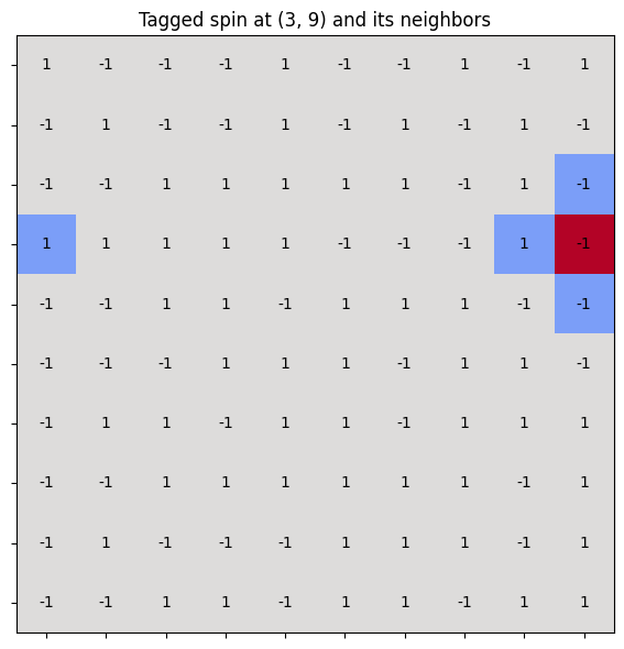
• In the Ising model with periodic boundary conditions, the modulo operation is used to wrap around the edges of the lattice—so that spins on one edge interact with those on the opposite edge.

• This effectively turns a 2D grid into a torus (doughnut shape), avoiding edge effects and mimicking an infinite system.

• Consider a 2D lattice of size $L\times L$. For a site at position $(i,j)$, its right neighbor is at $(i,j+1)$. But if $j=L-1$, then $j+1$ exceeds the lattice. To wrap around, we use:

• This brings the index back to $0$ when it exceeds $L-1$.

L = 10  # Lattice size
spins = np.random.choice([-1,1], size=(L, L))

i, j = 3, 9  # Current spin

# Neighbors with periodic boundary conditions
right = spins[i][(j + 1) % L]
left  = spins[i][(j - 1) % L]
up    = spins[(i - 1) % L][j]
down  = spins[(i + 1) % L][j]

Show code cell source Hide code cell source

import numpy as np
import matplotlib.pyplot as plt

# Create a color map: default to gray, highlight tagged spin and neighbors
color_map = np.full((L, L), 0.5)  # Gray background

# Highlight neighbors (green) and tagged spin (red)
color_map[i, j] = 1.0  # Red for the tagged spin

color_map[i, (j + 1) % L] = 0.2  # Green-ish
color_map[i, (j - 1) % L] = 0.2
color_map[(i - 1) % L, j] = 0.2
color_map[(i + 1) % L, j] = 0.2

# Plotting
fig, ax = plt.subplots(figsize=(6, 6))
im = ax.imshow(color_map, cmap="coolwarm", origin="upper", vmin=0, vmax=1)

# Overlay spin values
for x in range(L):
    for y in range(L):
        spin = spins[x, y]
        ax.text(y, x, f"{spin}", ha='center', va='center', color='black', fontsize=10)

# Grid and labels
ax.set_xticks(np.arange(L))
ax.set_yticks(np.arange(L))
ax.set_xticklabels([])
ax.set_yticklabels([])
ax.set_title(f"Tagged spin at ({i}, {j}) and its neighbors", fontsize=12)
ax.grid(False)

plt.tight_layout()
plt.show()

def get_dE(spins, i, j, J=1, B=0):
    '''Compute change in energy of 2D spin lattice 
    after flipping a spin at a location (i,j)''' 
    
    N = len(spins)
    
    z  = spins[(i+1)%N, j] + spins[(i-1)%N, j] + \
             spins[i, (j+1)%N] + spins[i, (j-1)%N] 
             
    dE = 2*spins[i,j]*(J*z + B)
    
    return dE

Generating chains! Master Equation and Detailed Balance#

Random chain

• In simple MC each sampled state $X_i$ at step $i$ is independet of the next or previous steps.

• Thus, MC sampling generates totally uncorrelated samples which is good for rapid convergence according to Central Limit Theorem. But as we remarked above the samples are most likely not covering important areas!

Markov chain:

• In simple MCMC each sampled state $X_i$ at steo $i$ is generated from $i-1$.

• This introduces correlations between samples which means slower covnergence to the mean.

• On the other hand MCMC find the important areas for sampling much faster so in the hand it wins big compared to MC.

• The probability of picking state $i+1$ given taht we started from $i$ is referred to as transition probability $T_{ij}$

• As a probability it should be normalized:

• Probability of being at $X$ at $t+\mathrm{\Delta }t$ given a prior state at $(X^{\prime },t)$ can be written in terms of $T_{X{X}^{\prime }}$ as:

• Subtracting P(X,t) from both states we can obtain equation of motion for Markov chain.

• Defining transition rates as the limit of $w_{X^{\prime }X}=li{m}_{\mathrm{\Delta }t\to 0}\frac{T_{X^{\prime }X}(\mathrm{\Delta }t)}{\mathrm{\Delta }t}$ we arrive at the master equation”

From maset equation we see that in order to reach equilibrium probability must stop depending on time. There are two possibilities:

• When the sum is equl zero becasue influx and outflux of probabiity currents cancel each out. This corresponds to steady state condition and is not true equilbroum for there are macroscopic fluxes in the system.

• When every single pairs is identically zero, this is known as detailed balance condition which is equivalent to thermodynamic equilibrium.

Master equation for a two state dynamics

• In the equilibrium we see that equilibrium is established when probability ratio matches the ratio of tranistions $\frac{p_1}{p_2}=\frac{w_{12}}{w_{21}}$

• In the $NVT$ ensemble we have an explicit requirment for transition rates $\frac{p_1}{p_2}=e^{-\beta (E_1-E_2)}=\frac{w_{12}}{w_{21}}$

How to pick the moves for Markov chain?#

• Now it is time to consider practical aspects of conducting MCMC. How to pick states and transitions?

• We have great freedom in picking states and moves as long as we satisfy the detailed balance! E.g as long as the ratio of transition probabilities matches ration of Botlzman factors!

• The simplest case for move is to pick one spins at random per iteration:

• For transitions we adopt criteria that favors our chain to explore low energy (high probability) configurations:

• If $p(X^{\prime })<p(X),$ $A_{X^{\prime }X}=\frac{p(X^{\prime })}{p(X)}$

• If $p(X^{\prime })\ge p(X),$ $A_{X^{\prime }X}=1$

Code for running 2D ising MCMC Simulations#

• If numba is installed, uncomment to benfit from jit acceleration!

• To speed benchmarks to assess how long simulation would take

from numba import njit
import numpy as np
import ipywidgets as widgets

@njit
def compute_total_energy(spins, J, B):
    N = spins.shape[0]
    E = 0.0
    for i in range(N):
        for j in range(N):
            S = spins[i, j]
            neighbors = spins[(i+1)%N, j] + spins[i, (j+1)%N]
            E -= J * S * neighbors
            E -= B * S
    return E

@njit
def run_ising2d(N, T, J, B, n_steps, out_freq):
    """
    Blazing fast 2D Ising Metropolis MCMC.

    Parameters:
    N        : Lattice size (N x N)
    T, J, B  : Temperature, coupling, field
    n_steps  : Number of Monte Carlo steps
    out_freq : Frequency of measurements

    Returns:
    S_out    : List of sampled spin states (sparse)
    E_out    : Per-spin energy list
    M_out    : Per-spin magnetization list
    """

    spins = 2 * (np.random.rand(N, N) < 0.5) - 1
    E_t = compute_total_energy(spins, J, B)
    M_t = np.sum(spins)

    # Preallocate memory
    n_out = n_steps // out_freq
    S_out = np.empty((n_out, N, N), dtype=np.int8)
    E_out = np.empty(n_out)
    M_out = np.empty(n_out)

    k = 0  # Output index

    for step in range(n_steps):
        
        i = np.random.randint(N)
        j = np.random.randint(N)

        S = spins[i, j]
        neighbors = spins[(i+1)%N, j] + spins[(i-1)%N, j] + spins[i, (j+1)%N] + spins[i, (j-1)%N]
        dE = 2 * S * (J * neighbors + B)

        if dE <= 0 or np.random.rand() < np.exp(-dE / T):
            spins[i, j] = -S
            E_t += dE
            M_t += -2 * S

        if step % out_freq == 0:
            S_out[k] = spins
            E_out[k] = E_t / N**2
            M_out[k] = M_t / N**2
            k += 1

    return S_out, E_out, M_out

def plot_ising(i):
    
    fig, ax  = plt.subplots(ncols=3, figsize=(10,4))
    
    ax[0].pcolor(S[i])
    ax[1].plot(E)
    ax[2].plot(M)
    
    ax[0].set(ylabel='$i$', xlabel='j')
    ax[1].set(ylabel='$E$', xlabel='steps')
    ax[2].set(ylabel='$M$', xlabel='steps')
    fig.tight_layout()
    plt.show()

#Simulation Parameters
params = {'N':40,
          'J':1,
          'B':0, 
          'T': 4,
          'n_steps': 100000, 
          'out_freq': 10}

# Simulation
S, E, M = run_ising2d(**params)

np.array(S).shape, np.array(E).shape, np.array(M).shape

((10000, 40, 40), (10000,), (10000,))

widgets.interact(plot_ising, i =(0, params['n_steps']//params['out_freq']-1))

i

4999

<function __main__.plot_ising(i)>

Carry out explorative simulations#

• How do we know if the simulation has done enough sampling? How do we assess convergence and errors?

• Test the dependence of observables on system size.

• Test the dependence of observables on initital conditions.

• Vary intensive parameters, e.g., temperature and field strength. Investigate changes in observables such as magnetization, energy, susceptibility, heat capacity.

• Think about alternative ways of accelerating and enhancing the sampling.

Parameter sweeps#

#Simulation Parameters
params = {'N':40,
          'J':1,
          'B':0, 
          'T': 4,
          'n_steps': 1000000, 
          'out_freq': 10}

Ts = np.linspace(1, 4, 40) 
Es, Ms, Cs, Xs = [], [], [], []  

for T in Ts:
    
    params['T']=T
    
    S, E, M = run_ising2d(**params)

    # Save last 90% percent of data
    idx = int(len(E) * 0.1) 
    
    E = E[idx:]
    M = M[idx:]
    
    Es.append(np.mean(E))
    Ms.append(np.mean(M))
    
    Cs.append(np.var(E)/T**2) 
    Xs.append(np.var(M)/T)

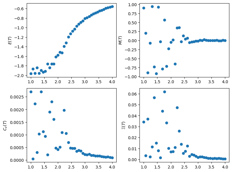
fig, ax  = plt.subplots(ncols=2, nrows=2, figsize=(8,6))

ax[0,0].scatter(Ts, Es)
ax[0,0].set(ylabel='$E(T)$')

ax[0,1].scatter(Ts, Ms)
ax[0,1].set(ylabel='$M(T)$')

ax[1,0].scatter(Ts, Cs)
ax[1,0].set(ylabel='$C_v(T)$')

ax[1,1].scatter(Ts, Xs)
ax[1,1].set(ylabel='$\Xi(T)$')
fig.tight_layout()

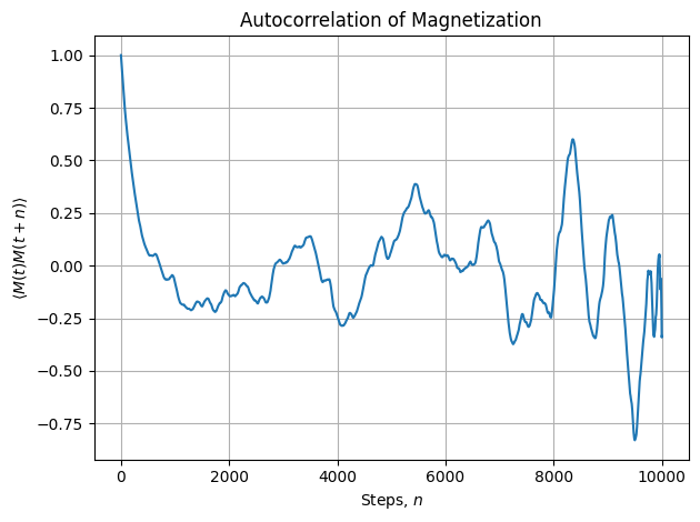
Autocorrelation functions#

• For any observable $A(t)$, you can compute:

• or the normalized version of autocorrelation funtion:

Integrated and exponential autocorrelation time#

• Once you compute $C(n)$, you can also estimate:

• Integrated autocorrelation time ${\tau }_{\text{int}}$: $${\tau }_{\text{int}}=\frac{1}{2}+\sum _{n=1}^{n_{\text{cut}}}\frac{C(n)}{C(0)}$$

• Exponential autocorrelation time by fitting $C(n)\sim \exp (-n/{\tau }_{\text{exp}})$

Show code cell source Hide code cell source

import numpy as np
import matplotlib.pyplot as plt
from scipy.optimize import curve_fit

def autocorr(x):
    """
    Computes the normalized autocorrelation function of a 1D time series x.

    Parameters:
    x : array-like
        Time series (e.g., magnetization over MC steps)

    Returns:
    acf : array-like
        Autocorrelation function normalized so that acf[0] = 1
    """
    n = len(x)
    x = x - np.mean(x)
    result = np.correlate(x, x, mode='full')[-n:]
    result /= x.var() * np.arange(n, 0, -1)
    return result

def exp_decay(n, a, tau):
    """Exponential decay model"""
    return a * np.exp(-n / tau)

def estimate_exp_autocorr_time(x, max_lag=100):
    """Estimate exponential autocorrelation time and effective sample size"""
    acf = autocorr(x)
    lags = np.arange(max_lag)

    # Fit exponential decay model to ACF
    try:
        popt, _ = curve_fit(exp_decay, lags, acf[:max_lag], p0=(1.0, 10.0))
        a, tau_exp = popt
    except RuntimeError:
        tau_exp = np.nan  # Fit failed

    # Compute effective sample size
    N_eff = len(x) / (2 * tau_exp) if tau_exp > 0 else np.nan

    # Plot
    plt.figure(figsize=(5, 3))
    plt.plot(lags, acf[:max_lag], label="Autocorrelation")
    plt.plot(lags, exp_decay(lags, *popt), '--', label=f"Fit: $\\tau_{{\\exp}}$ ≈ {tau_exp:.2f}")
    plt.xlabel("Lag")
    plt.ylabel("Autocorrelation")
    plt.legend()
    plt.tight_layout()
    plt.grid(True)
    plt.show()

    return tau_exp, N_eff

#Simulation Parameters
params = {'N':40,
          'J':1,
          'B':0, 
          'T': 4,
          'n_steps': 100000, 
          'out_freq': 10}

# Simulation
S, E, M = run_ising2d(**params)

# Example usage
#M = np.random.randn(1000)  # Replace with your magnetization time series
acorr = autocorr(M)

rho_t = acorr / acorr[0]

# Plotting
plt.plot(rho_t[:10000])
plt.xlabel('Steps, $n$')
plt.ylabel(r'$\langle M(t) M(t+n) \rangle$')
plt.title('Autocorrelation of Magnetization')
plt.grid(True)
plt.tight_layout()
plt.show()

# Example usage:
x = np.random.randn(1000).cumsum()  # Strongly correlated data
tau_exp, N_eff = estimate_exp_autocorr_time(x)

print(f"Exponential autocorrelation time: {tau_exp:.2f}")
print(f"Effective sample size: {N_eff:.1f} (out of {len(x)} total samples)")

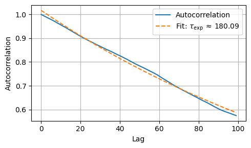
Exponential autocorrelation time: 187.41
Effective sample size: 2.7 (out of 1000 total samples)

Problems#