Markov Chains#
import numpy as np
import matplotlib.pyplot as plt
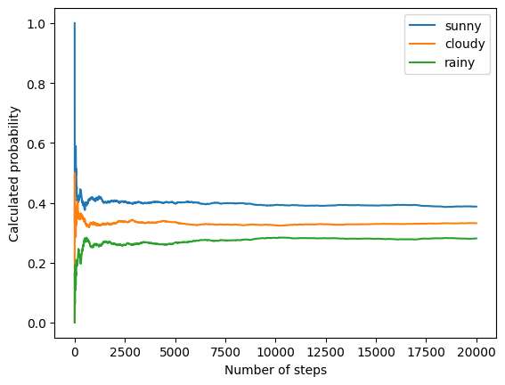
The Markov chain will hop around on a discrete state space which is made up from three weather states:
state_space = ("sunny", "cloudy", "rainy")
In a discrete state space, the transition operator is just a matrix. Columns and rows correspond, in our case, to sunny, cloudy, and rainy weather. We pick more or less sensible values for all transition probabilities:
transition_matrix = np.array(((0.6, 0.3, 0.1),
                              (0.3, 0.4, 0.3),
                              (0.2, 0.3, 0.5)))
n_steps = 20000
states = [0]

for i in range(n_steps):
    states.append(np.random.choice((0, 1, 2), p=transition_matrix[states[-1]]))

states = np.array(states)
fig, ax = plt.subplots()
width = 1000
offsets = range(1, n_steps, 5)

for i, label in enumerate(state_space):
    p_offest=[np.sum(states[:offset] == i) / offset for offset in offsets]
    ax.plot(offsets, p_offest, label=label)

ax.set_xlabel("Number of steps")
ax.set_ylabel("Calculated probability")
plt.legend()
<matplotlib.legend.Legend at 0x7f6b0415fee0>
Example of detailed balance: Isomerisation reaction#
To illustrate the approach to equilibrium in a reversible A ↔ B reaction using a Markov chain model, let’s consider the following scenario and Python simulation:
Scenario Setup In this chemical interconversion reaction:
\(A \rightarrow B\) with probability \(p\)
\(B \rightarrow A\) with probability \(q\)
Markov Chain Model
The system has two states (A, B), with transitions defined by a transition matrix.
Simulate Transitions: The simulation determines the system’s state after each step by following the transition probabilities.
Calculate Equilibrium: We observe how the system’s state probabilities evolve over \(N\) steps to reach equilibrium.
impot numpy as np
# Transition probabilities
p = 0.3  # Probability of going from A to B
q = 0.7  # Probability of going from B to A

# Transition matrix
transition_matrix = np.array([
    [1-p, p],  # From A to A, B
    [q, 1-q]   # From B to A, B
])

# Initial state (0 for A, 1 for B)
current_state = 0

# Number of steps to simulate
n_steps = 1000

# Record the state at each step to visualize the approach to equilibrium
state_history = np.zeros((n_steps, 2))  # Create a history record for both states A and B
state_history[0, current_state] = 1

# Simulate the Markov chain
for step in range(1, n_steps):
    current_state = np.random.choice([0, 1], p=transition_matrix[current_state])
    state_history[step, current_state] = 1

# Calculate cumulative probabilities over time to show how probabilities stabilize
cumulative_probabilities = np.cumsum(state_history, axis=0) / np.arange(1, n_steps+1).reshape(-1, 1)
  Cell In[6], line 1
    impot numpy as np
          ^
SyntaxError: invalid syntax
# Plotting the results
fig, (ax1, ax2) = plt.subplots(nrows=2)
ax1.plot(cumulative_probabilities[:, 0], label='Probability of A', color='blue')
ax1.plot(cumulative_probabilities[:, 1], label='Probability of B', color='red')
ax1.set_xlabel('Steps')
ax1.set_ylabel('Probability')
ax1.set_title('Approach to Equilibrium Probabilities of States A and B')
ax1.legend()
ax1.grid(True)


# Plotting the results
ax2.bar(['A', 'B'], [state_record[0]/n_steps, state_record[1]/n_steps], color=['blue', 'red'])
ax2.set_ylabel('Probability')
ax2.set_title('Equilibrium probabilities of states A and B')
fig.tight_layout()
As the number of steps increases, the fraction of time the system spends in each state \(A\) and \(B\) should converge to the theoretical equilibrium probabilities. These are derived from the detailed balance conditions \(p \cdot \pi_A = q \cdot \pi_B\) and the normalization condition \(\pi_A + \pi_B = 1\).
This simulation visually demonstrates the concept of reaching equilibrium in a reversible reaction through a Markov process, which is essential in understanding statistical thermodynamics.