Mean Field

What You Will Learn

• The Mean Field Approximation (MFA) simplifies complex systems by replacing fluctuating variables with their average values.

• When applied to functions of many interacting variables, MFA assumes that correlations can be neglected:

\[ \langle f(x_1, x_2, x_3, \dots) \rangle \approx f(\langle x_1 \rangle, \langle x_2 \rangle, \langle x_3 \rangle, \dots) \]

• This approximation is foundational across many areas of physics, including:

  • Electronic structure theory (e.g., Hartree–Fock)

  • Liquid state theory (e.g., van der Waals)

  • Condensed matter physics (e.g., Ising and Heisenberg models)

MFA applied to the Ising Model

• In the Ising model, the mean-field approximation (MFA) decouples spin–spin interactions, reducing the system to a single macroscopic parameter: the average magnetization per spin, denoted by \( m \).

\[ \langle s_i s_j \rangle \approx \langle s_i \rangle \langle s_j \rangle = m^2 \]

\[ \langle H \rangle \approx -J \sum_{\langle ij \rangle} \langle s_i \rangle \langle s_j \rangle - h \sum_i \langle s_i \rangle = -\frac{1}{2} J q m^2 - h m \]

• The factor of \( \frac{1}{2} \) avoids double-counting spin pairs, and \( q \) is the coordination number—for instance, \( q = 4 \) for a 2D square lattice and \( q = 6 \) for a 3D cubic lattice.

Derivation of the Mean-Field Hamiltonian

• Consider the 2D Ising model where each spin \( s_i \) interacts with its \( q \) nearest neighbors:

\[ H_i = -J \sum_{\delta} s_i s_{i+\delta} - h s_i = -\left( J \sum_{\delta} s_{i+\delta} + h \right) s_i \]

• Define the local mean field at site \( i \) as:

\[ H_i^{\text{MF}} = J \sum_{\delta} s_{i+\delta} + h \]

• Under the mean-field approximation, replace neighboring spins with their average value:

\[ H_i^{\text{MF}} \approx J q m + h \]

• The total Hamiltonian then becomes:

\[ H \approx - (J q m + h) \sum_i s_i \]

• Taking the thermal average and accounting for double counting leads to the previously derived mean-field expression for \( \langle H \rangle \).

Self-Consistent Equation for Magnetization

• Partition Function: After applying MFA, the system becomes effectively non-interacting, and the total partition function factorizes as \( Z = z^N \), where \( z \) is the partition function of a single spin. For \( s_i = \pm 1 \):

\[ E(s_i = \pm 1) = \mp (J q m + h) \]

\[ z = e^{\beta (J q m + h)} + e^{-\beta (J q m + h)} \]

• The probability that a spin is in state \( s_i \) is:

\[ p(s_i) = \frac{e^{\beta s_i (J q m + h)}}{z} \]

• Average Magnetization: The mean value of a spin is then:

\[ m = \langle s_i \rangle = \sum_{s_i} s_i \, p(s_i) = \frac{e^{\beta (J q m + h)} - e^{-\beta (J q m + h)}}{e^{\beta (J q m + h)} + e^{-\beta (J q m + h)}} \]

\[ m = \tanh(\beta (J q m + h)) \]

• This self-consistent equation relates the average magnetization \( m \) to itself via the hyperbolic tangent function, capturing the thermal competition between spin alignment and disorder.

Free Energy of Mean-Field Ising Models

Defining the Macrostate \( M \)

• Consider a spin lattice of \( N \) sites, where each spin can point up or down. The total magnetization is given by:

\[ N = N_{+} + N_{-}, \qquad M = N_{+} - N_{-} \]

• Defining the magnetization per spin \( m = M/N \), the probabilities of spin-up and spin-down states are:

\[ p_{\pm} = \frac{1 \pm m}{2} \]

Entropy, Energy, and Free Energy

• Entropy is given by the Shannon expression using the probabilities of spin states:

\[ S(m) = -N k_B \left[ \left( \frac{1+m}{2} \right) \log \left( \frac{1+m}{2} \right) + \left( \frac{1-m}{2} \right) \log \left( \frac{1-m}{2} \right) \right] \]

• Energy in the mean-field approximation is the sum over spins in the presence of an average field:

\[ E(m) = -N \left[ \frac{Jq}{2} m^2 + h m \right] \]

• Free Energy is the usual Legendre transform:

\[ F(m) = E(m) - T S(m) \]

• Dimensionless Free Energy per Spin (useful for analysis and plotting):

\[ f(m) = \frac{F}{N k_B T} = - \left[ \frac{Jq}{2 k_B T} m^2 + \frac{h}{k_B T} m \right] + \left[ \left( \frac{1+m}{2} \right) \log \left( \frac{1+m}{2} \right) + \left( \frac{1-m}{2} \right) \log \left( \frac{1-m}{2} \right) \right] \]

Finding the Critical Temperature \( T_c \)

• The critical point is determined by the second derivative of the free energy:

\[ \frac{\partial^2 f}{\partial m^2} \bigg|_{m=0} = 1 - \frac{Jq}{k_B T} = 0 \]

\[ \Rightarrow \quad T_c = \frac{Jq}{k_B} \]

Magnetization as a Function of Temperature

• The equilibrium magnetization minimizes the free energy, leading to a self-consistency condition:

\[ m = \tanh \left( \frac{Jq}{k_B T} m + \frac{h}{k_B T} \right) \]

• Rearranged as:

\[ - \left( \frac{Jq}{k_B T} \right) m - \frac{h}{k_B T} + \tanh^{-1}(m) = 0 \]

• For zero external field (\( h = 0 \)), the equation simplifies to:

\[ m = \tanh \left( \frac{T_c}{T} m \right) \]

• For small \( m \), expand \( \tanh^{-1}(m) \approx m + \frac{1}{3} m^3 \), yielding:

\[ - \frac{T_c}{T} m + m + \frac{1}{3} m^3 = 0 \]

• Solving this, we find the magnetization near the critical point behaves as:

\[ m = \pm \sqrt{ \frac{3(T_c - T)}{T_c} } \]

Visualizing MF predictions

The \(h=0\) MFA case

The equation can be solved in a self-consistent manner or graphically by finding intersection between:

• \(m =tanh(x)\)

• \(x = \frac{Jqm}{k_BT}\)

When the slope is equal to one it provides a dividing line between two behaviours.

\[k_B T_c =qJ\]

\[m = tanh \Big(\frac{Tc}{T} m \Big)\]

• MFA shows phase-transition!

import ipywidgets as widgets
from ipywidgets import interactive, interact
import matplotlib.pyplot as plt
import numpy as np

# Constants
J = 1  # Interaction strength
k = 1  # Boltzmann constant (set to 1 for simplicity)

def entropy(m):
    # Handle log of zero by adding a small number to the argument
    small_number = 1e-10
    return -(1+m)/2 * np.log((1+m)/2 + small_number) - (1-m)/2 * np.log((1-m)/2 + small_number)

def free_energy(m, T):
    # Calculate the free energy for given m and T
    return -0.5 * J * m**2 - T * entropy(m)

def plot_free_energy(T):
    # Magnetization range
    m_values = np.linspace(-1, 1, 100)
    F_values = [free_energy(m, T) for m in m_values]
    
    # Plotting
    plt.figure(figsize=(8, 5))
    plt.plot(m_values, F_values, label=f'T = {T}')
    plt.xlabel('Magnetization (m)')
    plt.ylabel('Free Energy per Spin (F)')
    plt.title('Mean-field Free Energy vs. Magnetization')
    plt.legend()
    plt.grid(True)
    plt.show()

interactive(plot_free_energy, T=(0.1, 2, 0.1 ))

def mfa_ising_Tc(T=1, Tc=1):

    x  = np.linspace(-3,3,1000)
    
    f = lambda x: (T/Tc)*x
    m = lambda x: np.tanh(x)
    
    plt.plot(x,m(x), lw=3, alpha=0.9, color='green')
    
    plt.plot(x,f(x),'--',color='black')
    idx = np.argwhere(np.diff(np.sign(m(x) - f(x))))
    plt.plot(x[idx], f(x)[idx], 'ro')
    
    plt.legend(['m=tanh(x)', 'x'])
    
    plt.ylim(-2,2)
    plt.grid('True')
    plt.xlabel('m',fontsize=16)
    plt.ylabel(r'$tanh (\frac{Tc}{T} m )$')
    plt.show()

import plotly.graph_objects as go
import numpy as np
from scipy.optimize import fsolve
from scipy.optimize import root_scalar  # Importing root_scalar

def compute_xcross(T, h_over_T):
    
    def f(M):
        Tc = 1.0  # Normalized temperature
        h = h_over_T * T  # Compute actual h from h/T and T
        return M - np.tanh((M + h) / (T / Tc))
    
    # Using symmetric interval for root finding to allow negative solutions
    interval = [-2.0, 2.0]

    # Check if a root is likely within the given range
    if f(interval[0]) * f(interval[1]) > 0:
        return 0.0  # If no root likely, return 0
    
    # Find the root using bisection method within the specified range
    result = root_scalar(f, bracket=interval, method='bisect')
    
    return result.root 

# Define ranges for h/T  and T/Tc (from 0.2 to 1.5)
h_over_T_values = np.linspace(-0.2, 0.2, 101)
T_over_Tc_values = np.linspace(0.1, 1.6, 101)

# Create a meshgrid for T/Tc and h/T
H_over_T, T_over_Tc = np.meshgrid(h_over_T_values, T_over_Tc_values)

# Initialize an array for magnetizations
Magnetizations = np.zeros_like(H_over_T)

# Compute M for each (h/T, T/Tc) pair in the meshgrid
for i, T in enumerate(T_over_Tc_values):
    for j, h in enumerate(h_over_T_values):
        
        Magnetizations[i, j] = compute_xcross(T, h)


# Create a 3D surface plot using Plotly
fig = go.Figure(data=[go.Surface(z=Magnetizations, x=H_over_T, y=T_over_Tc, 
                                 colorscale='RdBu', 
                                 contours={
                                     #'z': {'show': True, 'start': -1.0, 'end': 1.0, 'size': 0.1, 'color':'orange'},
                                     'x': {'show': True, 'start': -1, 'end': 1, 'size': 0.05, 'color':'black'},
                                     'y': {'show': True, 'start': 0.5, 'end': 1.5, 'size': 0.1, 'color':'black'}
                                 })])

# Update plot layout
fig.update_layout(
    title='3D Plot of Magnetization M vs normalized temperature and field; T/Tc and h/T',
    scene=dict(
        xaxis_title='h/T',
        yaxis_title='T/Tc',
        zaxis_title='M',
        aspectmode='manual',
        yaxis_autorange='reversed',  # Reverse the Y-axis
        aspectratio=dict(x=2, y=2, z=0.75),  # Adjust these values as needed
        camera=dict(
            eye=dict(x=-4, y=-2, z=2),  # Adjust camera "eye" position for better view
            up=dict(x=0, y=0, z=1)  # Ensures Z is up
        )
    ),
    autosize=False,
    width=900,
    height=900
)

# Display the figure with configuration options
fig.show()

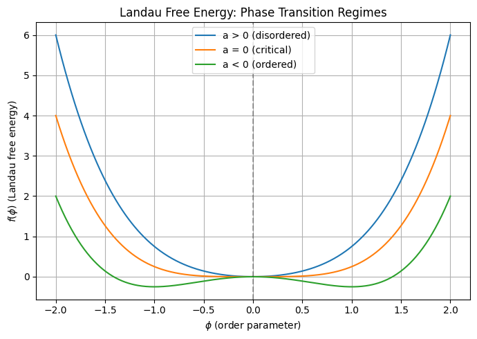
Landau Theory

Show code cell source Hide code cell source

import numpy as np
import matplotlib.pyplot as plt

# ==== Free energy ====
def f(phi, a, b):
    return 0.5 * a * phi**2 + 0.25 * b * phi**4

# ==== Range of phi ====
phi = np.linspace(-2, 2, 500)
b = 1.0  # fixed positive b

# ==== Plot for different 'a' ====
a_values = [1.0, 0.0, -1.0]
labels = ['a > 0 (disordered)', 'a = 0 (critical)', 'a < 0 (ordered)']
colors = ['#1f77b4', '#ff7f0e', '#2ca02c']

plt.figure(figsize=(7, 5))

for a, label, color in zip(a_values, labels, colors):
    plt.plot(phi, f(phi, a, b), label=label, color=color)

plt.axvline(0, color='k', linestyle='--', alpha=0.3)
plt.xlabel(r'$\phi$ (order parameter)')
plt.ylabel(r'$f(\phi)$ (Landau free energy)')
plt.title('Landau Free Energy: Phase Transition Regimes')
plt.legend()
plt.grid(True)
plt.tight_layout()
plt.show()

Show code cell source Hide code cell source

import numpy as np
import matplotlib.pyplot as plt
from matplotlib.animation import FuncAnimation
from IPython.display import HTML

# ==== Parameters ====
N = 128             # Grid size
dx = 1.0            # Spatial resolution
dt = 0.01           # Time step
steps = 1000        # Total time steps
save_every = 10     # Frame interval for animation
epsilon = 1.0       # Interfacial width parameter

# ==== Free energy parameters ====
a = -1.0   # linear coefficient (controls stability of φ = 0)
b = 1.0    # non-linear coefficient (typically > 0 to stabilize)

# ==== Landau free energy derivative ====
def f_prime(phi):
    return a * phi + b * phi**3

# ==== Laplacian with periodic boundary ====
def laplacian(field):
    return (
        -4 * field
        + np.roll(field, 1, axis=0) + np.roll(field, -1, axis=0)
        + np.roll(field, 1, axis=1) + np.roll(field, -1, axis=1)
    ) / dx**2

# ==== Initialize field ====
phi = np.random.rand(N, N) * 0.2 - 0.1  # small noise around 0

# ==== Store frames ====
frames = []

# ==== Simulation loop ====
for step in range(steps):
    mu = -epsilon**2 * laplacian(phi) + f_prime(phi)
    phi += dt * laplacian(mu)
    
    if step % save_every == 0:
        frames.append(phi.copy())

# ==== Animation ====
fig, ax = plt.subplots(figsize=(5, 5))
im = ax.imshow(frames[0], cmap='bwr', vmin=-0.05, vmax=0.05)

ax.axis('off')

def update(frame):
    im.set_array(frame)
    return [im]

ani = FuncAnimation(fig, update, frames=frames, interval=50, blit=True)
plt.close()  # avoid double display
HTML(ani.to_jshtml())

Once Loop Reflect