Final Project: Phase Separation in Binary Lennard-Jones Mixtures#
Background#
Many soft materials—such as polymer blends, lipid membranes, and even biological condensates—undergo phase separation when composed of two or more types of molecules. Whether a mixture remains homogeneous or separates into distinct domains depends on interaction strengths, temperature, and composition.
In this project, you will simulate a 2D (or 3D) binary mixture of LJ particles—types A and B—and investigate how varying parameters leads to mixing or phase separation.
You’ll explore:
How particle identity affects interaction potentials
How composition and temperature influence morphology
How to construct a phase diagram from simulation data
Project Goals#
Implement binary Lennard-Jones simulations of A/B particles
Study how tuning interspecies interaction (\( \varepsilon_{AB} \)) affects mixing
Identify when and how phase separation occurs
Estimate a phase diagram in the temperature–composition plane
Tasks#
1. Modify MD Code for Binary System#
Introduce two particle types: A and B.
Define three interaction strengths:
\( \varepsilon_{AA} = 1.0 \)
\( \varepsilon_{BB} = 1.0 \)
\( \varepsilon_{AB} = \) tunable parameter (e.g., 0.3–1.2)
Use the same \( \sigma \) for simplicity, or explore asymmetric sizes.
Tip: Maintain an array of particle types, and loop over all particle pairs to assign the correct LJ parameters.
2. Initialize Mixtures#
Start with a random mixture of A and B particles (e.g., 50/50 composition).
Use periodic boundary conditions and equilibrate for a long time.
3. Visualize and Detect Phase Separation#
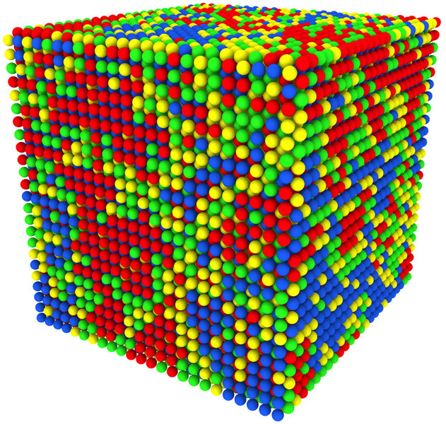
Visualize particle positions, coloring A and B differently.
At low \( T \) and low \( \varepsilon_{AB} \), you should observe domain formation (e.g., A-rich and B-rich regions).
At high \( \varepsilon_{AB} \) or high \( T \), the system should remain mixed.
4. Scan Parameters and Construct a Phase Diagram#
Run simulations at various:
Temperatures (e.g., from 0.5 to 2.0 in LJ units)
Compositions (e.g., from 20:80 to 80:20 A:B)
\( \varepsilon_{AB} \) values (e.g., 0.3 to 1.2)
For each combination, record whether the system appears mixed or phase separated (by visual inspection or density profiles).
Plot a phase diagram in the temperature–composition plane for a fixed \( \varepsilon_{AB} \), showing the boundary between mixed and demixed regions.
5. Challenges (Optional)#
Measure radial distribution functions \( g_{AA}(r) \), \( g_{AB}(r) \), \( g_{BB}(r) \)
Extract structure factor \( S(k) \) to quantify ordering length scale
Use clustering algorithms to identify domain size distributions
Simulate in 3D or use anisotropic particles (e.g., dumbbells)
Learning Outcomes#
Understand microscopic origins of demixing in multi-component systems
Learn how intermolecular forces determine macroscopic phase behavior
Develop skills in parameter scanning and phase diagram construction
Explore techniques for visualization and qualitative assessment of structure
Suggested Parameters#
Parameter |
Typical Value |
|---|---|
\( N \) |
100–500 |
\( \varepsilon_{AA}, \varepsilon_{BB} \) |
1.0 |
\( \varepsilon_{AB} \) |
0.3–1.2 |
\( \sigma \) |
1.0 |
Time step |
0.001–0.005 |
\( T \) |
0.5–2.0 |
Composition |
A:B from 20:80 to 80:20 |


