
Harmonic Oscillator#
What you need to know
In this section we study quantum mechanical version of harmonic oscillator. Harmonic oscillators have ubqiutuous presence in everyday world: beads bound by a spring which vibrate around equilibirum positions. Turns out beads on a pring is remarkably common in microsocpic world as nuclie of atoms in solids or molecules are in some sense “quantum beads” vibrating around equilibriu position of “quantum springs”. The distinction between quantum vs classical regimes will again be highly illuminating about the role of quantum effects on small scales. The key topics we will learn are:
Quantization of vibrations in molecules. Vibrational degrees of freedom are quantized which has implications for infrared and raman spectroscopies and bonding.
Existence of zero point energy and tunneling. Enenergy is not zero even at zero temperature. We appreciate this as a consequence of uncertainty relation.
Hermite Polynomials are eigenfunctions
Effects of unharmonicity. We will see the impact on energy levels of harmonic oscillators when one goes beyond harmonic approximation.
Raising and lower operators offer an elegant way of solving harmonic oscilator problem This will be our first introduction to raising and lowering operators which provide highly elegant way of solving problems in quantum mechanics.
Bead, spring and a wall.#
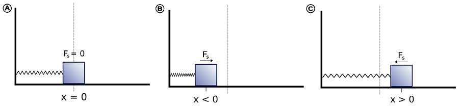
The classical harmonic oscillator is a system of bead attached to a wall with a spring. When bead is displaced from its equilibrium or resting position \(r_0\) to some point \(r\), experiences a restoring force \(F\) proportional to the displacement \(x=r-r_0\):
The above expression is also known as Hooke’s law, where minus sign indicates that the direction of force is always towards restoring equilibrium location. The constant k characterizes stiffness of the spring and is called spring constant.

Solving harmonic oscillator problem#
The classical equation of motion for a one-dimensional simple harmonic oscillator with a particle of mass m attached to a spring having spring constant k generates mechanical waves.
The intorduced constant \(\omega\) will be seen as the frequency oscillations.Note that frequency is inversly porportional to mass (heavier objects with same spring constant oscillate rapdily around equilibrium) and proprotional to spring constant (stiffer springs increase oscillations around equilibrium for same mass)
The differneital equation is a simple second order, linear ODE which can be solved by a standard trick of pluggin exponential \(x(t)=e^{\alpha t}\) and convertin the problem to algebraic equation. The solution is
The two constnants are: \(A\) the amplitude of oscillations and \(\phi\) is constant specifying the initial position of the bead.
Energy of the harmonic oscillator#
In classical mechanics the force and the potential energy of a conservative system are related via the formula:
This means the steeper the potential the higher the force and minus sign indicates that force is restoring the equilibrium position. The potential energy can be obtained by integrating:
Thus the potential energy for a simple harmoncin oscillator is a parabolic function of displacement. It is convenient to set \(C=0\) and measure potential energy relative to equilibrium state \(V(x=0)=0\)
The total energy consisting of kinetic and potential enregies will be used to obtain Schordinger equation.
Conservative system#
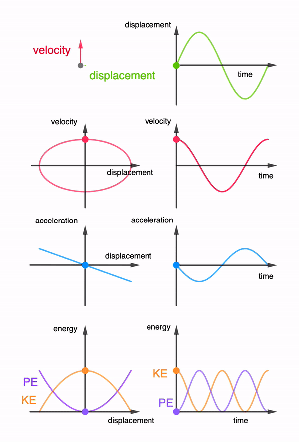
Fig. 19 The harmonic oscilator (in a vacuum) is a conservative system becasue the kinetic and potential energies keep being interconverted with no amount of total energy being dissipated into the environment. Oscillations go on forever with position \(x(t)\) velocity \(v=\dot{x}(t)\) and acceleration \(a=\ddot{x(t)}\) with same constant frequency \(\omega\) but with different amplitudes.#
Diatomic molecule and two-body problem#
Diatomic molecule is stable because the same force is acting on both ends
By expressing equations of motion in terms of the center of mass which, we find that center of mass moves freely without acceleration.
Next by taking difference between coordinates \(\ddot{x_2}=-\frac{k}{m_2}x_2\) and \(\ddot{x_1}=\frac{k}{m_1}x_1\)we expres the equations of motion in terms of relative distance
This equation looks identical to the probem of bead anchored to wall with a spring. We have thus managed to reduce the two body probelm to a one modey problem by replacing masses of bodies with a reduced mass: \(\mu=\frac{1}{m_1}+\frac{1}{m_2}=\frac{m_1 m_2}{m_1+m_2}\)
Beads and springs model of molecules#
Before discussing the harmonic oscillator approximation let us reflect on when this would be a good approximation and uner which cirumstances it will break down? For an aribtarry potential energy funciton of x we can carry out Taylor’s expansion around equilibrium bond length \(x_0\) obtaining infinitey series.
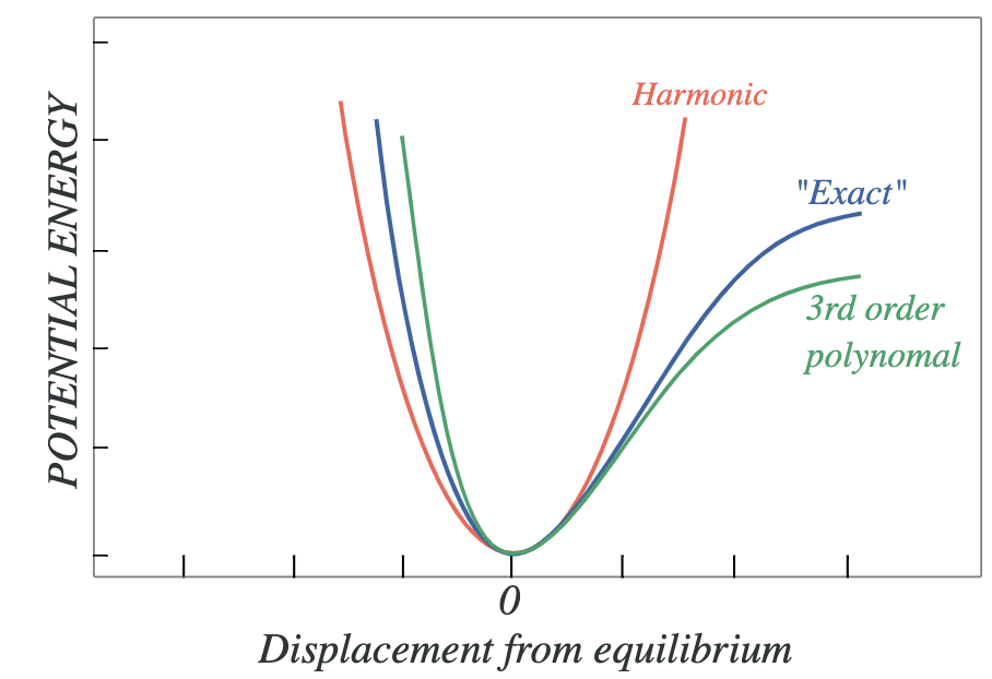
Fig. 20 Deviation from simple harmonic potential approximation (red curve) of true/exact potential (blue curve) with cubic term (green)#
Setting energy scale to be relative to \(U(x_0)=0\) and recongizing that first derivative vanishes at minima \(x_0\) we have
Hence we see that the Harmonic approximation is only the first non vanishing term! Furthermore we see that spring constant k and subsequent anharmonicity consnats such as \(\gamma\) are higher order derivatives of potential energy. That is the more non-linear the potential the higer the contribution of these terms. And vice verse clsoer the potential to quadratic form the more accurate is the harmonic assumtion.
Quantum harmonic oscillator#
Taking the classical Hamiltonian for a harmonic oscillator is given by:
The quantum mechanicalm harmonic oscillator is obtained by replacing the classical position and momentum by the corresponding quantum mechanical operators
Note that the potential term may be expressed in terms of three parameters becasue of \(k=\frac{\mu}{\omega}\) and \(\omega=2\pi \nu\) relations
\(k\) |
Force constant (kg \(s^{-2}\)) |
|---|---|
\(\omega\) |
Angular frequency (\(\omega = 2\pi\nu\); Hz) |
\(\nu\) |
Frequency (Hz; do not confuse this with quantum number \(v\)) |
Depending on the context any of these constants may be used to specify the harmonic potential.
Eigenfunctions and Eiganvalues#
The solutions to this equation produce eiganvalues (Energies)
Eigenfunctions (position wavefunctions)
Normalization factor \({N_v = \frac{1}{\sqrt{2^vv!}}\left(\frac{\alpha}{\pi}\right)^{1/4}}\)
where \(H_v\)’s are called Hermite polynomials.
n |
Hermite Polynomial \(( H_n(x))\) |
|---|---|
0 |
\(1\) |
1 |
\(2x\) |
2 |
\(4x^2 - 2\) |
3 |
\(8x^3 - 12x\) |
4 |
\(16x^4 - 48x^2 + 12\) |
For example, the wavefunctions for the two lowest states are:
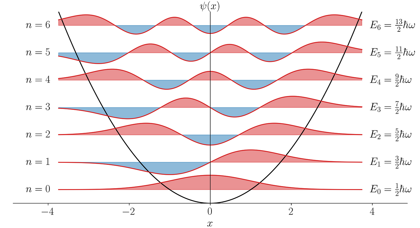
Fig. 21 Eigenfunctions and Eigenvalues of Harmonic Oscillator#
Interpreting solutions#
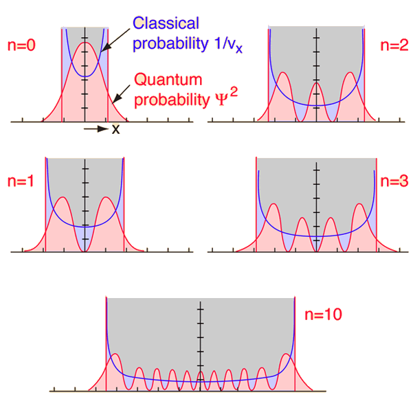
Fig. 22 Classical vs quantum probabilities of finding oscillating particle at position x#
Some of the lowest state solutions to the harmonic oscillator (HO) problem are displayed below:
Solutions \(\psi_v\) with \(v = 0, 2, 4, ...\) are even: \(\psi_v(x) = \psi_v(-x)\).
Solutions \(\psi_v\) with \(v = 1, 3, 5, ...\) are odd: \(\psi_v(x) = -\psi_v(-x)\).
Integral of an odd function from \(-a\) to \(a\) (\(a\) may be \(\infty\)) is zero.
The tails of the wavefunctions penetrate into the potential barrier deeper than the classical physics would allow. This phenomenon is called quantum mechanical tunneling.
Hermite Polynomials#
The following realtions are useful when working with Hermite polynomials:
Examples#
Example
Show that the lowest level of Harmonic oscillator obeys the uncertainty principle.
Solution
First we calculate \(\left<\hat{x}\right>\) (\(\psi_0\) is an even function, \(x\) is odd, the integrand is odd overall):
For \(\left<\hat{x}^2\right>\) we have (integration by parts or tablebook):
For \(\left<\hat{p}_x\right>\) we have again by symmetry:
Note that derivative of an even function is an odd function. For \(\left<\hat{p}_x^2\right>\) we have:
Finally, we can calculate \(\Delta x\Delta p_x\):
Recall that the uncertainty principle stated that: \(\Delta x\Delta p_x \ge \frac{\hbar}{2}\)
Thus we can conclude that \(\psi_0\) fulfills the Heisenberg uncertainty principle.
Example
Quantization of nuclear motion. Molecular vibration in a diatomic molecule can be approximated by the quantum mechanical harmonic oscillator model. There \(\mu\) is the reduced mass as given previously and the variable \(x\) is the distance between the atoms in the molecule (or more exactly, the deviation from the equilibrium bond length \(R_e\)).
a. Derive the expression for the standard deviation of the bond length in a diatomic molecule when it is in its ground vibrational state.
b. What percentage of the equilibrium bond length is this standard deviation for carbon monoxide in its ground vibrational state? For \(^{12}C^{16}O\), we have: \(\tilde{v}\) = 2170 cm\(^{-1}\) (vibrational frequency) and \(R_e\) = 113 pm (equilibrium bond length)
Solution
The harmonic vibration frequency is given in wavenumber units (\(cm^{-1}\)). This must be converted according to: \(\nu = c\tilde{v}\). The previous example gives expression for \(\sigma_x\):
In considering spectroscopic data, it is convenient to express this in terms of \(\tilde{v}\):
In part (b) we have to apply the above expression to find out the standard deviation for carbon monoxide bond length in its ground vibrational state. First we need the reduced mass:
The standard deviation is now:
Harmonic Oscillator in 3D#
In a three-dimensional harmonic oscillator the potential energy term now can have different spring constants corresponding to deformation along each axis:
the separation of variables technique similar to the three-dimensional particle in a box problem can be used here. The result is once again eigenfunctions that are product of 1D eigenfunctions and eigenvalues that are sum of 1D eigenvalues:
The \(\alpha\), \(N\), and \(H\) are defined in above and the \(v\)’s are the quantum numbers along the Cartesian coordinates.