Schrödinger Equation

What you need to know

• By combining the classical wave equation with quantum principles, we derive a new equation that describes quantum wave functions: Schrödinger’s Equation (SE).

• Schrödinger’s Equation, like the classical wave equation, depends on both time and space.

• We can apply the method of separation of variables to transform the time-dependent Schrödinger equation (TD-SE) into the time-independent Schrödinger equation (TI-SE). The time-independent form is especially important in the chemical and biological sciences, and it will be our primary focus for the remainder of the course.

• We will introduce the operator notation, a powerful mathematical framework that allows us to express the equations of quantum mechanics in a concise and elegant form.

• In quantum mechanics, every physical quantity that can be measured experimentally—such as energy, momentum, or position—has a corresponding operator.

• We will reformulate the process of solving Schrödinger’s equation into finding the eigenfunctions and eigenvalues associated with these operators, which represent measurable quantities in quantum systems.

The exciting journey into the microscopic world.

• In the next few sections, we will introduce Schrödinger’s Equation (SE), one of the fundamental laws of physics. A “fundamental law” means that SE cannot be derived from more basic principles; it can only be inferred or hypothesized based on experimental evidence. Its validity is supported by countless successful quantitative predictions and explanations of experimental observations.

• It’s important to emphasize that there has never been an instance where quantum mechanics has failed when applied correctly. The physical world is inherently quantum, especially at small scales. Quantum mechanics works flawlessly—at all scales and in all situations where it has been properly applied.

Fig. 46 You are now entering the quantum world. Proceed wih caution

What we require from the new quantum theory?

• Recall that while classical mechanics is valid at large scales, it completely fails to describe motion at the atomic and molecular levels. A new, accurate equation of motion is required to explain phenomena such as:

  • The quantized nature of energy, as observed in experiments involving blackbody radiation and atomic and molecular spectra.

  • Wave-particle duality, demonstrated through electron diffraction, Compton scattering, and double-slit experiments.

Fig. 47 Schrodinger had to make peace with the idea that correct description of electrons is done via wave functions.

Quantum wave equation

• In 1925/1926 Erwin Schrödinger, who was an expert on physics of waves, derived a new equation of motion which allows computing, predicting and obtaining from first principles the quantum phenomena such as energy quantization and wave-particle duality.

• We can trace Schordinger’s approach by starting with classical wave equation

  \[\frac{\partial^2 \Psi(x,t)}{\partial x^2}=\frac{1}{v^2}\frac{\partial^2 \Psi(x,t)}{\partial t^2}\]

• The classical wave equation we have seen can produce waves which can be traveling or standing depending on boundary conditions. Lets pick a general periodic traveling wave for instance

\[\Psi(x,t) = Ae^{i(kx-\omega t)}\]

• We are going to plug into a wavefunction the two key quantum relations discovered emprically and then see what kind of wave equation can produce

  • Plug wave-particle duality via De Broglie relation:

  \[p=h/\lambda=\hbar k\,\,\,\, where\,\,\,\, k=\frac{2\pi}{\lambda}\]

  • Plug energy quantization via Planck equaton:

  \[E=h\nu=\hbar\omega\,\,\,\, where\,\,\,\, \omega=2\pi\nu\]

• Quantum wave function

\[\Psi(x,t)=Ae^{\frac{i}{\hbar}(px-E t)}\]

• What equation can genereate such quantum wave functions? To find out we need to take derivatives with respect to time and space.

From Quantum Wave Function to Quantum Wave Equation

• Time Part: When we take the time derivative of the wave function, we find that the total energy appears as a multiplicative factor. This is significant because, in quantum mechanics, total energy is conserved. The relationship between energy and the time dependence of the wave function is given by:

\[ \frac{\partial \Psi(x,t)}{\partial t} = -\frac{i}{\hbar} E \Psi(x,t) \]

• Spatial Part: To recover the total energy from the spatial part of the wave function, we take two spatial derivatives.

\[ \frac{\partial \Psi(x,t)}{\partial x} = \frac{i}{\hbar} p \Psi(x,t) \]

\[ \frac{\partial^2 \Psi(x,t)}{\partial x^2} = -\frac{p^2}{\hbar^2} \Psi(x,t) = -\frac{2m(E - V)}{\hbar^2} \Psi(x,t) \]

• This equation where variable of time is absent is time-independent schordinger equation. Will come back to it shortly.

• Joining time and spatial parts by expressing the kinetic energy as a difference between total and potential energies \(K = E-V\) and eliminating \(E\) we get:

Time-Dependent Schrödinger Equation

\[ -\frac{\hbar^2}{2m} \frac{\partial^2 \Psi}{\partial x^2} + V(x) \Psi = i \hbar \frac{\partial \Psi}{\partial t} \]

Quantum vs Classical Wave equation

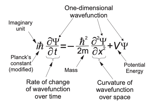
Fig. 48 Diseecting Schordinger Equation (using 1D version for simplicity).

• Schoridnger equation describes spatial evolution of wave function \(\Psi(x,t)\) for a quantum system like an electron or atom in a potential \(V(x)\).

• Unlike classical wave equation there is only single time derivative! The presence of \(i\) generates oscillatory solutions in complex planes hence why we call it quantum wave equation.

• What is the meaning of \(\Psi(x,t)\)? It is generaly complex hence can’t stand for any real measruable quantity. Will see how to extract infromation from \(\Psi\) later.

• Note we are focusing on 1D case for simplicity. Generalizing to 3D invlves adding up similiar terms that depend on \(y\) and \(z\) coordinates of every quantum object.

Separation of Variables and Time Indepdendent Schrodinger Equation

• By assuming the wave function can be separated into a product of a spatial part and a time part, \(\Psi(x,t) = \psi(x) T(t)\), we can solve for each part independently:

• The time part \(T(t)=e^{-iEt/\hbar}\) yields an oscillatory solution related to the total energy.

• The spatial part \(\psi(x)\) satisfies the time-independent Schrödinger equation, which we solve to obtain stationary states.

Quantum Wave function

\[\Psi(x,t) = \psi(x)\cdot e^{-iEt/\hbar}\]

• The hard part is finding \(\psi(x)\) which depends on the system, e.g form of poteantial energy function \(V\)

• This method is crucial for solving quantum systems, particularly in cases where the potential \(V(x)\) does not depend on time.

• Plugging \(\psi(x) T(t)\) and cancelling time part we are back to the time-independent equation that we had gotten earlier.

Time-Independent Schrödinger Equation

\[ -\frac{\hbar^2}{2m} \frac{\partial^2 \psi}{\partial x^2} + V(x) \psi = E \psi \]

The Mathematical Language of Quantum Mechanics: Operators

• To streamline our discussion and draw analogies with classical intuition, we need to introduce some essential notation and terminology.

• In quantum mechanics, we define operators as mathematical entities that transform one function into another. An operator can perform various actions on a function, such as differentiation, integration, addition, multiplication, and more. In this way, operators serve as tools to manipulate wave functions and extract physical information.

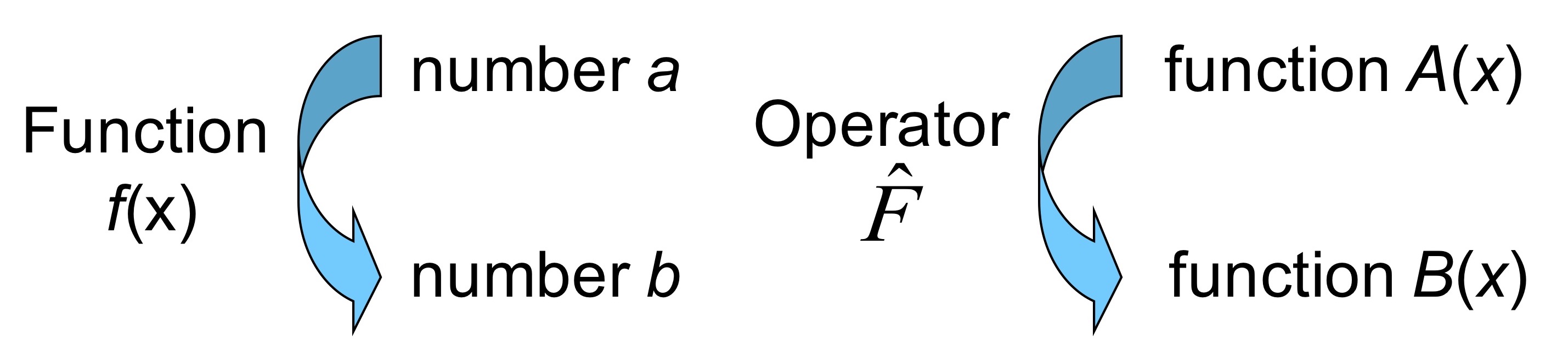
Fig. 49 Analogy of operators with ordinary functions.

Example of operators

• Lets take a function e^{2x} as an example and see how operator notation works:

\[\frac{d^2}{dx^2} e^{2x} = 4e^{2x}\]

\[\hat{A} f =4f\]

• Where we say that operator \(\hat{A}\) acts on function \(e^{2x}\) to produce another function which in this case is same function multiplied by 4.

• In general operators can be anything in front of function \(f(x)\), here are a few more examples of operators :

  • \(\hat{A}f = x\) multiplies function by x, e.g \(\hat{A}e^{2x} = xe^{2x}\)

  • \(\hat{A} = -i\) multiplies function by \(-i\), e.g \(\hat{A}e^{2x} = -ie^{2x}\)

  • \(\hat{A} = \sqrt{}\), takes square root, e.g \(\hat{A}e^{2x} = e^{x}\)

  • \(\hat{A} = (d/dx +x^2)\), takes derivative then adds \(x^2\) multiplication \(\hat{A}e^{2x} = 4e^{2x}+x^2e^{2x} = (4+x^2)e^{2x}\)

Linear operators.

• Linear means that operator acting on sum of function does not change the power of any of functions.

\[\hat{A}[c_1 f_1(x)+c_2f_2(x)]= c_1 \hat{A}f_1(x)+c_2 \hat{A}f_2(x)\]

• Schrödinger equation is a linear differential equation. Hence it can be written as a linear operator acting on a wave function.

Example of linear operators

• Which of the following would be linear operator? \(\hat{A}=\frac{d}{dx}\), \(\hat{B}=\int dx\) \(\hat{C}=\sqrt{}\).

• Using rules of calculus we know that derivative and integral acts on each term in the sum:

\[\frac{d}{dx}(c_1f_1+c_2f_2) = c_1\frac{df_1}{dx}+c_2\frac{df_2}{dx}\]

\[\int(c_1f_1+c_2f_2)dx = c_1\int f_1dx+c_2\int f_2dx\]

• For the square root linear property does not hold!

\[\sqrt{(c_1f_1+c_2f_2)} \neq c_1\sqrt{f_1} +c_2\sqrt{f_2}\]

Schrödinger equation in operator notation.

• By expressing the equation in operator notation, we can start to recognize various terms and see that the Schrödinger equation, like any proper equation of motion, embodies the principle of total energy conservation:

• Lets take Schoridnger equation and denote differntials as operators acting on wavefunction. E.g lets look at two sides of itime dependent schrodinger equation: \( \left[ -\frac{\hbar^2}{2m} \frac{\partial^2 \Psi}{\partial x^2} + V(x) \right] \Psi \) and \(i\hbar \frac{\partial }{\partial t} \Psi\)

• The operator of the position part is called Hamiltonian Operator and it has a deep connection to energy conservation and Hamiltonian function of classical mechanics

Classical Hamiltonian:

\[ H(x,p) = K + V = \frac{p^2}{2m} + V(x) \]

• Classical Hamiltonian tepresents total energy showing us how kinetic and potential energy change as a function of momentum and position.

Quantum Hamiltonian:

\[ \hat{H} = \hat{K} + \hat{V} = -\frac{\hbar^2}{2m} \frac{\partial^2}{\partial x^2} + V(x) \]

• The operator \(\hat{H}\), known as the Hamiltonian operator, is the quantum mechanical analog of the classical Hamiltonian, which represents the total energy:

Schrödinger Equation in operator form

\[ \hat{H} \psi = E \psi \]

\[ \hat{H} \psi = i\hbar \frac{\partial \psi}{\partial t} \]

• Hamiltonian Operator: \(\hat{H}\) It can stand for 1D, 2D, or 3D systems and describe any quantum object from one electron to collection of molecules.

• Energy: Describes the possible energy states of the quantum system.

• Energy Operator: \(i\hbar \frac{\partial}{\partial t}\)

• Note how the potential energy term appears in the same form across different systems—it is always a function of spatial coordinates. Some examples of potentials

  • \(V(x) = 0\) represents a free particle,

  • \(V(x) = kx^2\) describes a particle trapped in a harmonic potential,

  • \(V(x) = \cos(x)\) corresponds to a particle in a periodic potential.

The correspondence principle of Quantum Mechanics

• Thanks to universality of energy conservation law, for every observable in classical mechanics there can be found a corresponding operator in quantum mechanics! Lets list them here:

Observables	Classical	Quantum
Position	\(x\)	\(\hat{x}=x\)
Momentum	\(p=mv\)	\(\hat{p}=-i\hbar \frac{\partial}{\partial x}\)
Potential Energy	\(V(X)\)	\(\hat{V}=V(x)\)
Kinetic Energy	\(K=\frac{p^2}{2m}\)	\(\hat{K}=\frac{\hat{p}^2}{2m}\)
Total Energy	\(H(x,p)=\frac{p^2}{2m}+V(x)\)	\(\hat{H}=\hat{K}+\hat{V}\)
Equation of motion	Newton’s law \(F=ma\) or Hamiltons equations	\(\hat{H}\psi=E\psi\) Or \(i\hbar\frac{\partial \psi}{\partial t}=\hat{H}\psi\)
Quantization and wave-particle duality?	N/A	Energy quantization and duality are naturally described by \(E_n\) and \(\psi_n\).

Linearity and Principle of supersposition

• As we recall from solving classical wave equation whenever there are boundary conditions imposed on the spatial domain of our PDE we can end up having infinite number of solutions \(u_n(x)\) discretized by integers \(n=1,2,...\) for each spatial coordinate.

• The general solution was written as linear combination of normal modes. Likewise boundary conditions produce infinite number of solutions to quantum wave equation discretized by intege numbers \(n\): \(\hat{H} \psi_n(x)=E_n \psi_n(x)\)

• The general solution is again written as linear combination of quatnum wave functions thanks to linearity of schrodinger equation:

\[\psi(x,t) = \sum_n c_n \psi_n(x) f_n(t)\]

Eigenvalues and Eigenfunctions

• In both the classical wave equation and the time-independent Schrödinger equation, we can use operator notation to frame the problem as one of finding special functions and their corresponding multiplicative factors that satisfy specific operators.

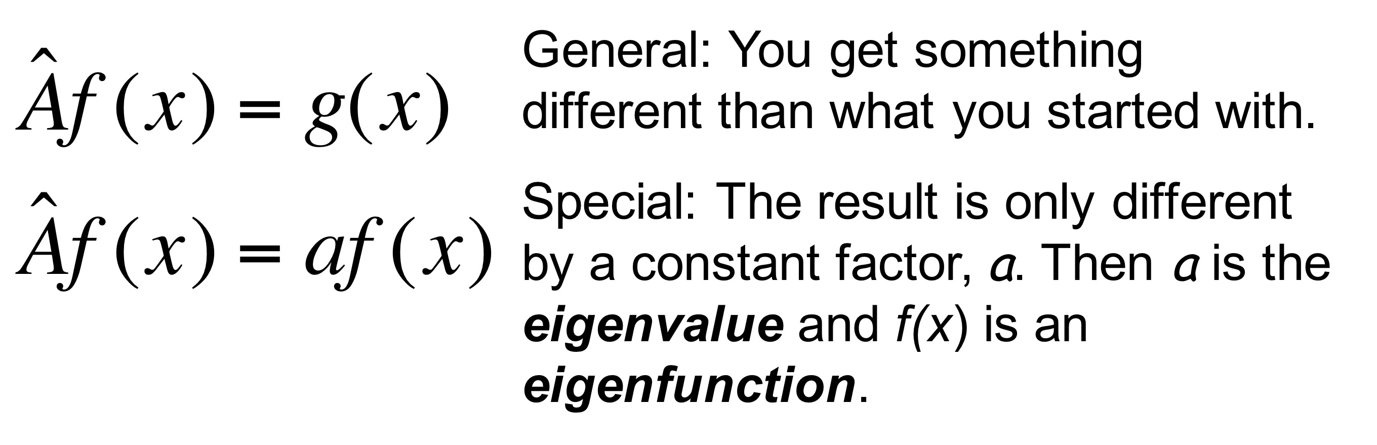
Fig. 50 Eigenvalue/Eigenfunction problem

• In general, the action of an operator can change a function, but in quantum mechanics, we are particularly interested in operators that preserve the form of the function, producing only a constant multiplicative factor.

• The time-independent Schrödinger equation can be viewed as an eigenfunction-eigenvalue problem, where the eigenfunctions

Schordinger Equation as Eigenfunctions/Eigenvalues problem

\[ \boxed{\hat{H} \psi_n = E_n \psi_n} \]

• \(\psi_n\) the wavefunctions are the eigenfunctions of Hamitonian operator

• \(E_n\) the energies are the eiganvalues of Hamiltonian operator

Problems

Problem 1

Confirm that the following wavefunctions are eigenfunctions of linear momentum and kinetic energy (or neither or both):

• \(C sin(ax)\)

• \(N e^{-ix/\hbar}\)

Solution

Start by applying linear momentum operator to first function:

\[-i \hbar \dfrac{\partial}{\partial x} A \sin(ax) = -i \hbar Aa \cos(ax) \nonumber\]

• We see that action of operator changed the \(sin\) function hence sin function can not be an eigenfunction of linear momentum.

Next we apply kinetic energy operator:

\[\begin{split} \begin{align*} -\dfrac{\hbar^2}{2m} \dfrac{\partial^2}{\partial x^2} A \sin(ax) &= -\dfrac{\hbar^2}{2m} \dfrac{\partial}{\partial x} Aa \cos(ax) \\[4pt] &= +\dfrac{\hbar^2}{2m} Aa^2 \sin(ax) \end{align*} \nonumber \end{split}\]

• Kinetic energy operator did not modify the function hence s\(sin\) function is an eigenfunction for kinetic energy operator

Problem 2: Taking the Square of an Operator

Consider the operator \( \hat{A} = x \frac{d}{dx} \). Find \( \hat{A}^2 \), i.e., \( \hat{A}(\hat{A}f(x)) \), and apply it to an arbitrary function \( f(x) \).

Solution

First, apply \( \hat{A} f(x) = x \frac{d}{dx} f(x) \):

\[ \hat{A} f(x) = x \frac{df}{dx} \]

Now, apply \( \hat{A} \) again to the result:

\[ \hat{A}(\hat{A} f(x)) = \hat{A} \left( x \frac{df}{dx} \right) = x \frac{d}{dx} \left( x \frac{df}{dx} \right) \]

Using the product rule:

\[ \frac{d}{dx} \left( x \frac{df}{dx} \right) = \frac{df}{dx} + x \frac{d^2 f}{dx^2} \]

Thus:

\[ \hat{A}^2 f(x) = x \left( \frac{df}{dx} + x \frac{d^2 f}{dx^2} \right) = x \frac{df}{dx} + x^2 \frac{d^2 f}{dx^2} \]

Problem 3: Verifying Eigenfunction and Eigenvalue

Consider the operator \( \hat{B} = -i\hbar \frac{d}{dx} \) (momentum operator). Verify that \( f(x) = e^{ikx} \) is an eigenfunction of \( \hat{B} \), and find the corresponding eigenvalue.

Solution

Apply \( \hat{B} \) to \( f(x) = e^{ikx} \):

\[ \hat{B} f(x) = -i\hbar \frac{d}{dx} e^{ikx} \]

The derivative of \( e^{ikx} \) is:

\[ \frac{d}{dx} e^{ikx} = ik e^{ikx} \]

Thus:

\[ \hat{B} f(x) = -i\hbar \cdot ik e^{ikx} = \hbar k e^{ikx} \]

Since \( \hat{B} f(x) = \hbar k f(x) \), \( f(x) = e^{ikx} \) is an eigenfunction of \( \hat{B} \) with eigenvalue \( \hbar k \).

Problem 4: Testing for an Eigenfunction and Eigenvalue

Given the operator \( \hat{C} = \frac{d^2}{dx^2} \) (second derivative operator), check if \( f(x) = e^{-\alpha x^2} \) is an eigenfunction of \( \hat{C} \), and find the eigenvalue if it is.

Solution

Apply \(\hat{C} = \frac{d^2}{dx^2} \) to \( f(x) = e^{-\alpha x^2} \):

\[ \frac{d}{dx} e^{-\alpha x^2} = -2\alpha x e^{-\alpha x^2} \]

Taking the second derivative:

\[ \frac{d^2}{dx^2} e^{-\alpha x^2} = \frac{d}{dx} \left( -2\alpha x e^{-\alpha x^2} \right) = -2\alpha e^{-\alpha x^2} + 4\alpha^2 x^2 e^{-\alpha x^2} \]

Thus:

\[ \hat{C} f(x) = \left( -2\alpha + 4\alpha^2 x^2 \right) e^{-\alpha x^2} \]

Since this is not proportional to \( f(x) = e^{-\alpha x^2} \), \( f(x) \) is not an eigenfunction of \( \hat{C} \).

Problem 5: Linearity and Eigenfunction Testing

Consider the operator \( \hat{D} = x^2 \frac{d}{dx} \). Show whether this operator is linear and check if \( f(x) = x^n \) is an eigenfunction of \( \hat{D} \).

Solution

First, test linearity by applying \( \hat{D} \) to \( \alpha f(x) + \beta g(x) \):

\[ \hat{D}(\alpha f(x) + \beta g(x)) = x^2 \frac{d}{dx} (\alpha f(x) + \beta g(x)) = \alpha x^2 \frac{df}{dx} + \beta x^2 \frac{dg}{dx} \]

This is \( \alpha \hat{D} f(x) + \beta \hat{D} g(x) \), so \( \hat{D} \) is linear.

Now, apply \( \hat{D} \) to \( f(x) = x^n \):

\[ \hat{D} f(x) = x^2 \frac{d}{dx} x^n = x^2 \cdot n x^{n-1} = n x^n \]

Since the result is proportional to \( f(x) = x^n \), \( f(x) = x^n \) is an eigenfunction of \( \hat{D} \) with eigenvalue \( n \).