DEMO: H wavefunctions

Requirements | Importing libraries

import numpy as np
import  matplotlib.pyplot as plt
import plotly.graph_objects as go
from scipy.special import sph_harm, genlaguerre, factorial

%matplotlib inline
%config InlineBackend.figure_format = 'retina'

try:
    from google.colab import output
    output.enable_custom_widget_manager()
    print('All good to go')
except:
    print('Okay we are not in Colab just proceed as if nothing happened')

Okay we are not in Colab just proceed as if nothing happened

1. Describing a radial function \(R_{nl}(r)\)

\[R_{nl} = \sqrt{ \Big( \frac{2}{n a_0} \Big)^3 \frac{(n-l-1)!}{2n(n+l)!}} \cdot e^{-\frac{r}{n a_0}} \cdot \Big( \frac{2 r}{n a_0} \Big)^l \cdot L^{2l+1}_{n-l-1}\Big( \frac{2 r}{n a_0} \Big)\]

def radial_function(r, 
                    n=1, 
                    l=0):
    '''Rnl(r) normalized radial function
    r: radial distance Float (0, inf)
    n: principal quantum number Int (1,2,3... inf)
    l: angular quantum number Int (0,1,2,... n-1)
    '''
    
    a0 = 1 # set Bohr radius to 1 (Hartree units)

    prefactor = np.sqrt( ((2 / n * a0) ** 3 * (factorial(n - l - 1))) / (2 * n * (factorial(n + l))) )

    laguerre = genlaguerre(n - l - 1, 2 * l + 1)

    p = 2 * r / (n * a0)
    

    return  prefactor * np.exp(-p / 2) * (p ** l) * laguerre(p)

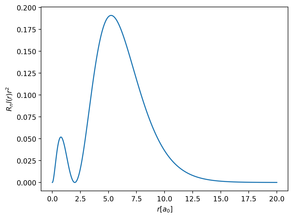
r = np.linspace(0, 20, 1000)

Rnl = radial_function(r, n=2, l=0)

#plt.plot(r, Rnl)
#plt.plot(r, Rnl**2)
plt.plot(r, r**2 * Rnl**2)
plt.xlabel(r'$r [a_0]$')
plt.ylabel(r'$R_nl(r) r^2$')

Text(0, 0.5, '$R_nl(r) r^2$')

Check properties of radial distributon functions

r = np.linspace(0, 100, 10000)
dr = r[1]-r[0]

Rnl = radial_function(r, n=5, l=3)

pr = r**2 * Rnl**2 

norm = np.trapz(pr * dr) # Check normalizaton
#cdf  = np.cumsum(pr * dr) 

print(norm)

0.9999999052314471

np.trapz(pr*r*dr)

2. Describing an angular function | Spherical harmonic \(Y_{l}^{m}(\theta, \varphi)\)

• We will make use of sph_harm function from Scipy

• We can also build up spherical harmonics using Associated Legendre function using lpvm

\[ Y_{lm}(\phi,\theta) = \sqrt{\frac{2l+1}{4\pi} \frac{(l-m)!}{(l+m)!} } P_{lm}(cos \phi) \cdot e^{im\theta} \]

sph_harm(0, 0, np.pi, np.pi) # test a few spherical harmonics

(0.28209479177387814+0j)

def plot_Yml(l, m):
    '''Visualizing spherical harmonics using sph_harm funcion from Scipy special function library
     Note that the name of angles is different from the notation adopted in QM textbooks!
     l: angular quantum number (0,1,2,...)
     m: magnetic quantum number (-l,...l)
     '''

    #Creade grid of phi and theta angles for ploting surface mesh
    phi, theta = np.linspace(0, np.pi, 100), np.linspace(0, 2*np.pi, 100)
    phi, theta = np.meshgrid(phi, theta)

    #Calcualte spherical harmonic with given m and l
    Ylm = sph_harm(m, l, theta, phi) 
    R=abs(Ylm)
    
    # Let's normalize color scale
    fcolors    = Ylm.real
    fmax, fmin = fcolors.max(), fcolors.min()
    fcolors    = (fcolors - fmin)/(fmax - fmin)

    # Since we want to plot on cartesian reference frame we will use cartesian coordiniates x, y, z using R as the absolute value of Yml
    # Try a plot without R part. 
    fig = go.Figure(data=[go.Surface(x=R*np.sin(phi) * np.cos(theta), 
                                     y=R*np.sin(phi) * np.sin(theta), 
                                     z=R*np.cos(phi), 
                                     surfacecolor=fcolors,
                                     colorscale='balance')])

    # Show the plot
    fig.update_layout(title=fr'$Y_{l, m}$', autosize=False,
                      width=700, height=700,
                      margin=dict(l=65, r=50, b=65, t=90)
    )
    fig.show()

plot_Yml(l=1, m=0)

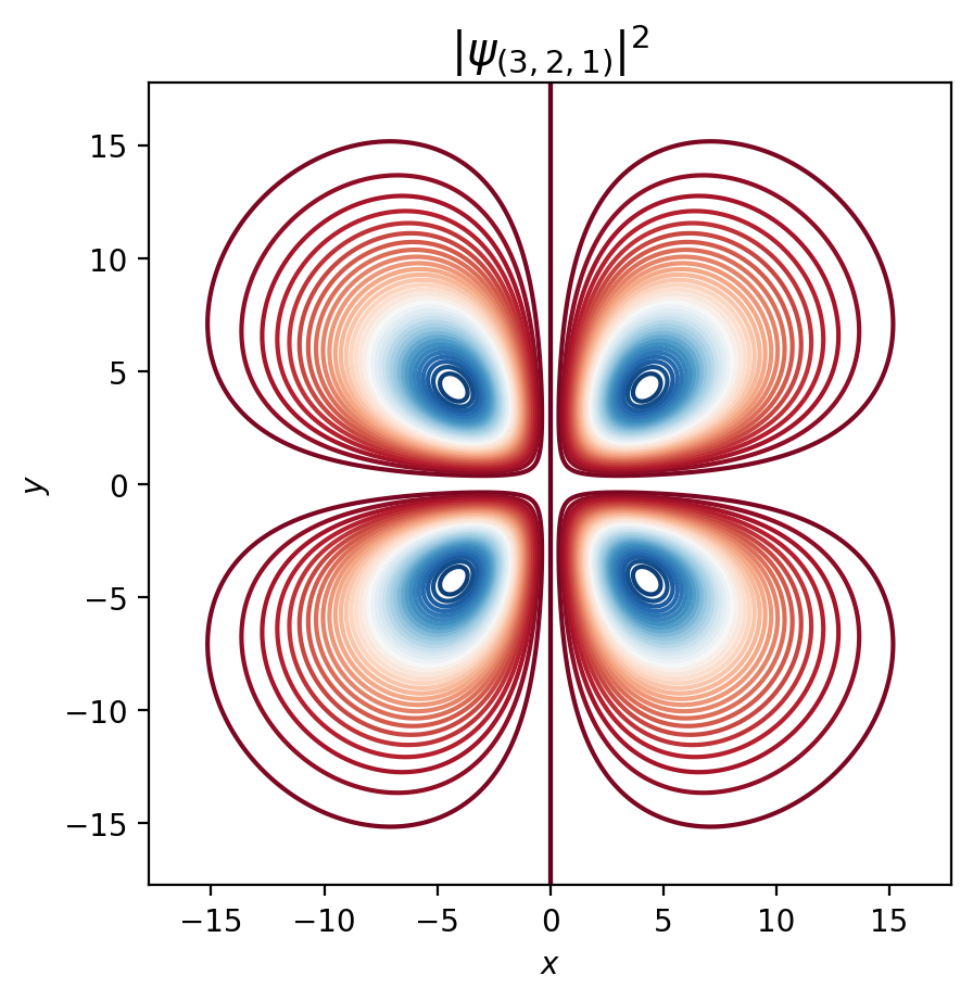
3. Describing the normalized probability as wavefunction squared \(|\psi _{nlm}(r,\theta ,\varphi)|^2\)

\[\psi_{nlm} = R_{nl}(r) \cdot Y_{l}^{m}(\theta, \varphi)\]

def normalized_wavefunction(n, 
                            l, 
                            m):

    '''Ψnlm(r,θ,φ) normalized wavefunction
    by definition of quantum numbers n, l, m and a bohr radius augmentation coefficient'''

    # Compute where radial function has nearly decayed to zero and determine cutoff distance
    r     = np.linspace(0, 500, 10000)
    pr = radial_function(r, n, l)**2 * r**2 * (r[1]-r[0])
    max_r = r[ np.where(np.cumsum(pr) >0.95)[0][0] ] 

    # Set coordinates grid to assign a certain probability to each point (x, y) in the plane
    x = y = np.linspace(-max_r, max_r, 501)
    x, y = np.meshgrid(x, y)
    r = np.sqrt((x ** 2 + y ** 2))

    # Ψnlm(r,θ,φ) = Rnl(r).Ylm(θ,φ)
    psi = radial_function(r, n, l) * sph_harm(m, l, 0, np.arctan(x / (y + 1e-7)))
    psi_sq = np.abs(psi)**2

    # Plot orbitals
    fig, ax = plt.subplots()
    ax.contour(psi_sq, 40, cmap='RdBu', extent=[-max_r, max_r,-max_r, max_r])
    ax.set_title(r'$|\psi_{{({0}, {1}, {2})}}|^2$'.format(n, l, m), fontsize=15)
    ax.set_aspect('equal')
    ax.set_xlabel(r'$x$')
    ax.set_ylabel(r'$y$')
    ax.set_xlim(-max_r, max_r)
    ax.set_ylim(-max_r, max_r)

normalized_wavefunction(n=3, 
                            l=2, 
                            m=1)

/tmp/ipykernel_25485/4170727653.py:22: RuntimeWarning: More than 20 figures have been opened. Figures created through the pyplot interface (`matplotlib.pyplot.figure`) are retained until explicitly closed and may consume too much memory. (To control this warning, see the rcParam `figure.max_open_warning`). Consider using `matplotlib.pyplot.close()`.
  fig, ax = plt.subplots()

The Kernel crashed while executing code in the the current cell or a previous cell. Please review the code in the cell(s) to identify a possible cause of the failure. Click <a href='https://aka.ms/vscodeJupyterKernelCrash'>here</a> for more info. View Jupyter <a href='command:jupyter.viewOutput'>log</a> for further details.

Full Atomic orbitals in 3D

xyz = np.linspace(-10, 10, 51)
x,y,z = np.meshgrid(xyz, xyz, xyz, sparse=False)

r = np.sqrt(x**2 + y**2 + z**2)
phi = np.arctan2(y+1e-10, x)
theta = np.where( np.isclose(r, 0.0), np.zeros_like(r), np.arccos(z/r) )

n,l,m=4,1,0
psi = radial_function(r, n, l) * sph_harm(m, l, phi, theta) 

/tmp/ipykernel_16723/2208657172.py:7: RuntimeWarning:

invalid value encountered in divide

/tmp/ipykernel_16723/1039204017.py:14: DeprecationWarning:

`np.math` is a deprecated alias for the standard library `math` module (Deprecated Numpy 1.25). Replace usages of `np.math` with `math`

fig= go.Figure(data=go.Isosurface(
    x=x.flatten(),
    y=y.flatten(),
    z=z.flatten(),
    value=abs(psi).flatten(),
    colorscale='RdBu',
    isomin=-.75*abs(psi).max(),
    isomax=.75*abs(psi).max(),
    surface_count=6,
    opacity=0.5,
    caps=dict(x_show=False,y_show=False,z_show=False)
))

fig.show()