
P5 Time dependence#
What you need to know
The time-dependent Schrödinger equation governs the evolution of quantum wave function over time \(\psi(x,t)\).
Stationary states are eigenfunctions of hamiltonian \(\hat{H}\) containing a spatial part and a time-dependent phase factor: \(\psi(x,t) = \psi(x) e^{-i E t / \hbar}\)
The stationary states have definite energy and their probability distributions are time-independent.
In more general situations, the wavefunction can be expressed as a linear superposition of energy eigenstates, with time evolution given by the phase factors of the eigenstates: \(\psi(x,t) = \sum_n c_n \psi_n(x) e^{-i E_n t / \hbar}\)
This superposition leads to time-dependent probabilities as different eigenstates interfere.
The time-dependence of quantum states is key to understanding quantum dynamics, such as oscillations between states in two-level systems or time evolution of quantum superpositions.
Time Dependence of a Pure Eigenfunction#
Until now, we have largely ignored the time dependence of quantum systems. This is because we have primarily focused on pure eigenfunction states, \(\psi_n(x,t)\), which exhibit no time-dependent behavior for observable quantities. The reason for this is straightforward:
In any probabilistic calculation, the time dependence vanishes because the expressions involve the square of the wavefunction. The absolute value of the complex time-dependent phase factor equals unity:
Similarly, for the expectation value of an operator \(\hat{A}\), the time-dependent phases cancel out, leaving only the spatial part:
Will we always have this fortunate cancellation of time dependence? The answer is no. When the system is described as a linear superposition of eigenstates, time dependence reappears in a significant way.
Time Dependence of a Superposition of Eigenfunctions#
Let us start with a superposition state of two energy eigenfunctions at time t=0:
What would the state be after some time t? By the virute of speration of variables we add the time dependence as a multiplicative factor for each eigenfunction:
Thus we see that the coefficients change over time. This means our state vector moves in functional space spanned by fixed orthogonal eigenfunctions! We can verify that the expression satisfies time-dependent Schrodinger equation by plugging it
Proof of superposition obeying Time dependent Schordinger Eq
Left hand side :
Right hand side:
Normalization is time independent!#
Certain quantities remain invariant under time evolution. For instance, it is natural to expect that normalization does not change over time—e.g., the particle must always be located somewhere within the box at any given moment.
The normalization condition is expressed as:
In the final step, we use the fact that the eigenfunctions are orthogonal, meaning \(\langle n \mid k \rangle = 0\) for \(n \neq k\), so the cross terms vanish and only the diagonal terms, where \(n = k\), survive.
Constants of Motion#
Quantities that remain conserved over time are called constants of motion. In quantum mechanics, we typically deal with expectations or averages rather than sharply defined values.
However, the principle of energy conservation dictates that the average total energy must be a conserved quantity. To determine whether a particular quantity depends on time, we take the time derivative of the expectation value:
\[\langle A \rangle = \langle \psi \mid \hat{A} \mid \psi \rangle\]The time derivative of this expectation value is:
\[ \frac{\partial}{\partial t}\langle A \rangle = \langle \frac{\partial \psi}{\partial t} \mid \hat{A} \mid \psi \rangle + \langle \psi \mid \hat{A} \mid \frac{\partial \psi}{\partial t} \rangle + \langle \psi \mid \frac{\partial \hat{A}}{\partial t} \mid \psi \rangle \]Now, using the time-dependent Schrödinger equation,
\[ i\hbar \frac{\partial}{\partial t} \mid \psi \rangle = \hat{H} \mid \psi \rangle \]we can express the time derivatives of the bras and kets as:
\[\langle \frac{\partial \psi}{\partial t} \mid = -\frac{1}{i\hbar} \langle \psi \mid \hat{H},\]\[\mid \frac{\partial \psi}{\partial t} \rangle = \frac{1}{i\hbar} \hat{H} \mid \psi \rangle.\]Substituting these into the time derivative of the expectation value, we obtain:
\[\frac{\partial}{\partial t}\langle A \rangle = \frac{1}{i\hbar} \langle \psi \mid \hat{A}\hat{H} \mid \psi \rangle - \frac{1}{i\hbar} \langle \psi \mid \hat{H}\hat{A} \mid \psi \rangle + \langle \psi \mid \frac{\partial \hat{A}}{\partial t} \mid \psi \rangle\]
Time dependence of expectation
This important relationship shows that if the operator \(\hat{A}\) does not explicitly depend on time, i.e., \(\frac{\partial \hat{A}}{\partial t} = 0\), then quantities that commute with the Hamiltonian \([\hat{A}, \hat{H}] = 0\) will be constants of motion. Those that do not commute, \([\hat{A}, \hat{H}] \neq 0\), will evolve over time.
Since the Hamiltonian commutes with itself and does not depend on time meaning that the energy is conserved.
\[ \frac{\partial}{\partial t}\langle E \rangle = 0 \]
Quantum Dynamics#

Fig. 55 Dynamics of wavefunction in the presence of gaussian potential. Show are square fo wavefunction along with its Real and imaginary components.#
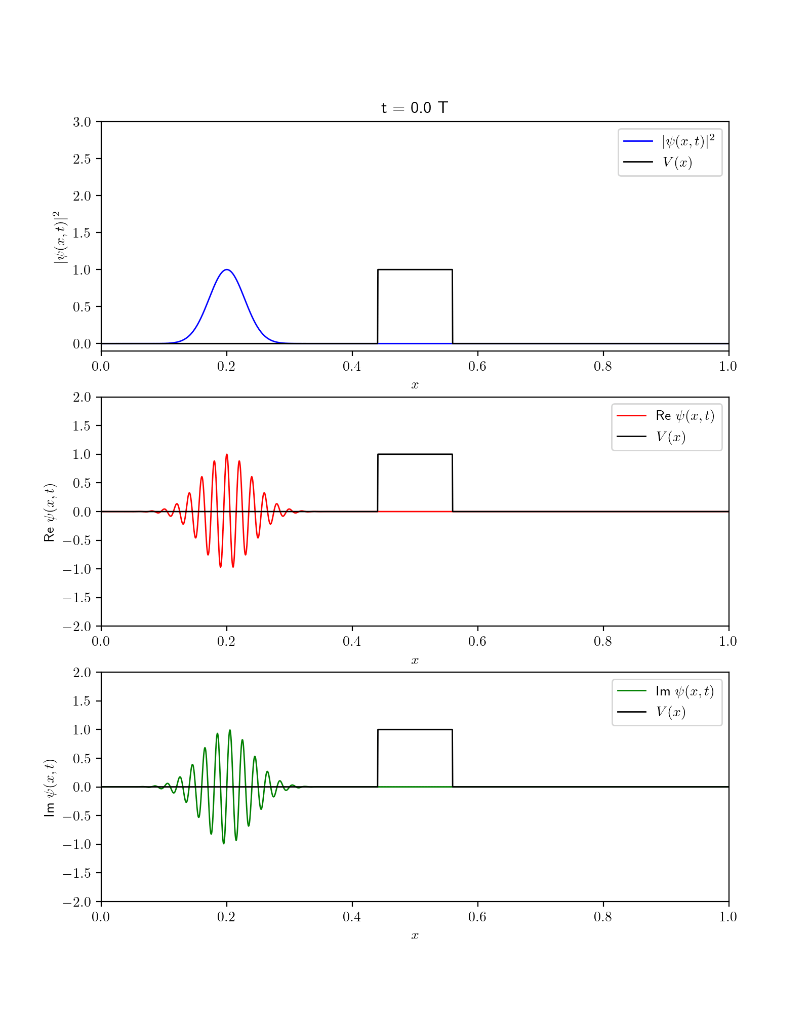
Fig. 56 Dynamics of wavefunction in the presence of barrier potential. Show are square fo wavefunction along with its Real and imaginary components.#