DEMO: Bonus challenge#
Quantum Waves
Prerequisites
Go over the demo notebook on quantum waves. You can copy paste and modify examples there to solve most challenges
Go over the python, numpy and matploltib basics to be more comfortable with the code.
How to complete the work
Run the cell below to import all necessary libraries.
Add code below each problem.
Run the code in Google Collab then download the file either as *.ipynb or *py file.
Submit your file to Canvas.
Do not forget that Google Collab deletes files if you do not save them iin your Google Drive.
import numpy as np
import matplotlib.pyplot as plt
from ipywidgets.widgets import interact, interactive

%matplotlib inline
%config InlineBackend.figure_format = 'retina'
Problem 1: Time independent PIB#
Evaluate the following quantities using particle in a box wavefunctions
Most likely to be in the middle thrid of box
Average momentum and momentum square
Average position and position square
Show uncertainty relation
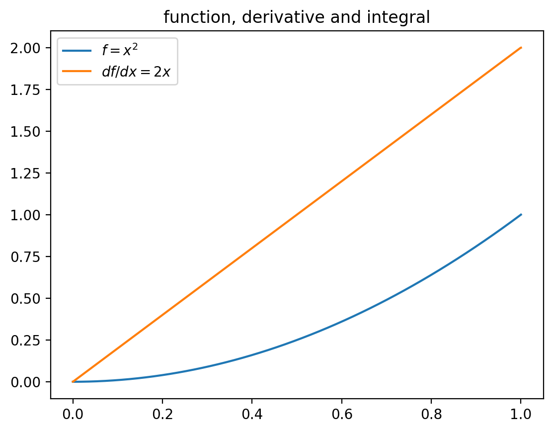
Hint: For some averages you may want to take numerical derivatives. Below is an example on how to do it using grad function of numpy. Also recall that numerically integral is just a sum over small discretized space dx. This is done by trapz function of numpy which is using trapezoidal rule
from  numpy import gradient as grad
from numpy import trapz

### Define boundaries and dx-
L  = 1
N  = 1000
dx = L/N
x  = np.linspace(0, L, N)

### A numerical array of function. Feel free to change this function, e.g exp or sine etc
f = x**2

plt.plot(x, f, label=r'$f=x^2$')

### First derivative function f(x)
dfdx = grad(f, x)

plt.plot(x, dfdx, label=r'$df/dx=2x$')

### Compute integral now using trapezoidal rule
int_f = np.trapz(dfdx, dx=dx)
print('Numerical integral:', int_f)

plt.legend()
plt.title('function, derivative and integral')
Numerical integral: 0.999
Text(0.5, 1.0, 'function, derivative and integral')
Problem 2: Time dependent PIB#
Compute time dependence of average position of a particle in a box as a linear combination of first two states weights.
Show the effect of changing second state into more excited states
Problem 3: Fourier transform and QM#
Fourier transform position wavefunction \(\psi(x)= \frac{1}{(2\pi \sigma^2)^{1/2}}\frac{}{}e^{-x^2/(2\sigma^2_x)}\) which will give you momentum wavefunction \(\psi(p)\).
Show uncertainty relation by varying sigma=0.1, 1, 10
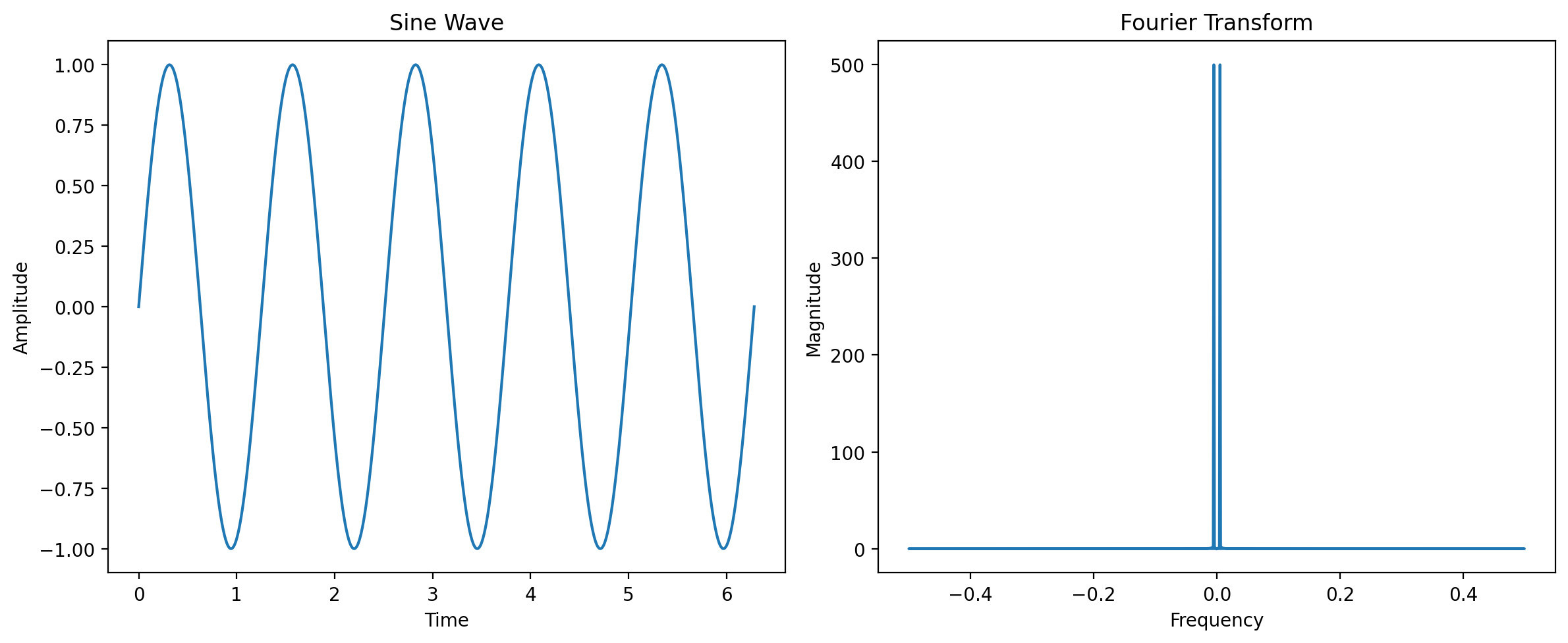
Below are two examples of Fourier transform
# Create a sine wave
x = np.linspace(0, 2*np.pi, 1000)
y = np.sin(5*x)

# Compute Fourier transform
Y = np.fft.fft(y)
frequencies = np.fft.fftfreq(len(Y))

# Plot
plt.figure(figsize=(12, 5))
plt.subplot(1, 2, 1)
plt.plot(x, y)
plt.title('Sine Wave')
plt.xlabel('Time')
plt.ylabel('Amplitude')

plt.subplot(1, 2, 2)
plt.plot(frequencies, np.abs(Y))
plt.title('Fourier Transform')
plt.xlabel('Frequency')
plt.ylabel('Magnitude')
plt.tight_layout()
plt.show()
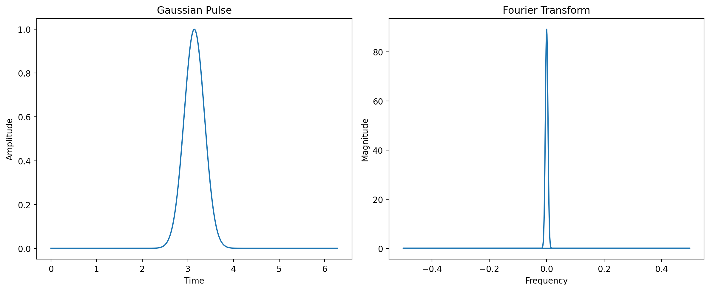
# Create a Gaussian pulse
y3 = np.exp(-(x-np.pi)**2/0.1)

# Compute Fourier transform
Y3 = np.fft.fft(y3)

# Plot
plt.figure(figsize=(12, 5))
plt.subplot(1, 2, 1)
plt.plot(x, y3)
plt.title('Gaussian Pulse')
plt.xlabel('Time')
plt.ylabel('Amplitude')

plt.subplot(1, 2, 2)
plt.plot(frequencies, np.abs(Y3))
plt.title('Fourier Transform')
plt.xlabel('Frequency')
plt.ylabel('Magnitude')
plt.tight_layout()
plt.show()