
DEMO: Quantum phenomena#
import numpy as np
import matplotlib.pyplot as plt


from scipy import constants as const
from scipy.constants import h, c, e, k, m_e, epsilon_0, Rydberg
# Rydberg constant in spec units

R_H_cm = Rydberg * 1e-2 # cm^-1

# Print to check
print("e =", e, "C")
print("h =", h, "J·s")
print("c =", c, "m/s")
print("ε0 =", epsilon_0, "F/m")
print("m_e =", m_e, "kg")
print("R_H =", R_H_cm, "cm^-1")
e = 1.602176634e-19 C
h = 6.62607015e-34 J·s
c = 299792458.0 m/s
ε0 = 8.8541878128e-12 F/m
m_e = 9.1093837015e-31 kg
R_H = 109737.3156816 cm^-1
Calculate wavelength of an electron#
Write a function to make calculations easier#
def rydberg_cm(n1, n2, Z=1):  # returns cm^-1

    return R_H_cm * Z**2 * (1/n1**2 - 1/n2**2)
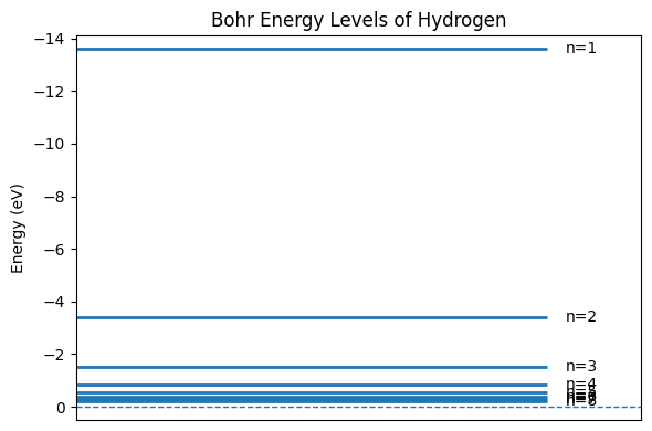
Plot sepctral transitions#
import numpy as np
import matplotlib.pyplot as plt

def plot_hydrogen_energy_levels(n_min=1, n_max=8):
    n_vals = np.arange(n_min, n_max + 1)
    E_eV = -13.6 / (n_vals ** 2)

    fig, ax = plt.subplots(figsize=(6, 4))
    for n, E in zip(n_vals, E_eV):
        ax.hlines(E, 0, 1, linewidth=2)
        ax.annotate(f"n={n}", xy=(1.01, E), xytext=(1.04, E),
                    textcoords="data", va="center", fontsize=10)

    ax.set_ylim(min(E_eV) - 0.5, 0.5)
    ax.invert_yaxis()
    ax.set_xlim(0, 1.2)
    ax.set_xticks([])
    ax.set_ylabel("Energy (eV)")
    ax.set_title("Bohr Energy Levels of Hydrogen")
    ax.axhline(0.0, linestyle="--", linewidth=1)  # ionization limit
    fig.tight_layout()
    return fig, ax

plot_hydrogen_energy_levels()
plt.show()
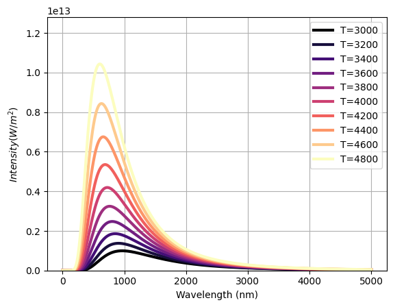
Plot Black Body radiation curves#
def planck(wavelength, T):
    """
    Planck's Law to calculate the spectral radiance of black body radiation at temperature T.

    Parameters:
    - wavelength (float): Wavelength in meters.
    - T (float): Absolute temperature in Kelvin.

    Returns:
    - (float): Spectral radiance in W/(m^2*sr*m).
    """

    exponent = (h*c) / (wavelength*k*T)

    exponent = np.clip(exponent, None, 700)  # Clip values of exponent at 700 to avoid numerical overflow

    return (2.0*h*c**2) / (wavelength**5 * (np.exp(exponent) - 1))


def plot_black_body(T, show=False):
    """
    Plot the black body radiation spectrum for a given temperature T.
    """

    # Lets pick some beautiful colors
    from matplotlib import cm
    from cycler import cycler
    magma = cm.get_cmap('magma', 10)  # 10 discrete colors, feel free to change
    plt.rcParams['axes.prop_cycle'] = cycler(color=[magma(i) for i in range(magma.N)])

    wavelengths = np.linspace(1e-9, 5e-6, 1000)  # Wavelength range from 1 nm to 3 um
    intensities = planck(wavelengths, T)

    plt.plot(wavelengths*1e9, intensities, label=f'T={T}', lw=3)  # Convert wavelength to nm for plotting

    plt.xlabel('Wavelength (nm)')
    plt.ylabel('$Intensity (W/m^2)$')
    plt.grid(True)
    plt.legend()

    max_int = max(planck(wavelengths, 5000)) # lets limit y axis to 5000
    plt.ylim(0, max_int)

    if show: # show is needed for interactive plots
        plt.show()
for T in range(3000, 5000, 200):
    plot_black_body(T)
/tmp/ipykernel_2234/3339301199.py:28: MatplotlibDeprecationWarning: The get_cmap function was deprecated in Matplotlib 3.7 and will be removed two minor releases later. Use ``matplotlib.colormaps[name]`` or ``matplotlib.colormaps.get_cmap(obj)`` instead.
  magma = cm.get_cmap('magma', 10)  # 10 discrete colors, feel free to change
from ipywidgets import interactive

interactive(plot_black_body, T=(1000, 5000, 100), show=True)
Dealing with complex numbers#
Consider the complex number \( z = 1 + \sqrt{3} i \).
import cmath # python provides special methods to convert between representtions
z=1+np.sqrt(3)*1j
z
(1+1.7320508075688772j)
z.real, z.imag
(1.0, 1.7320508075688772)
zc=z.conj()
np.sqrt(z*zc)
(1.9999999999999998+0j)
abs(z)
2.0
r, theta = cmath.polar(z)

r, theta
(2.0, 1.0471975511965976)
x, y = cmath.rect(r, theta)

x, y
---------------------------------------------------------------------------
TypeError                                 Traceback (most recent call last)
Cell In[15], line 1
----> 1 x, y = cmath.rect(r, theta)
      3 x, y

TypeError: cannot unpack non-iterable complex object
Complex numbers, Julia sets and fractals.#
Fractal is a mathematically defined, self-similar object which has similarity and symmetry on a variety of scales. The Julia Set Fractal is a type of fractal defined by the behavior of a function that operates on input complex numbers. More explicitly, upon iterative updating of input complex number, the Julia Set Fractal represents the set of inputs whose resulting outputs either tend towards infinity or remain bounded.
Julia set fractals are normally generated by initializing a complex number \(z = x + yi\) where \(i^2 = -1\) and x and y are image pixel coordinates in the range of about -2 to 2. Then, z is repeatedly updated using: \(z = z^2 + c\) where c is another complex number that gives a specific Julia set. After numerous iterations, if the magnitude of z is less than 2 we say that pixel is in the Julia set and color it accordingly. Performing this calculation for a whole grid of pixels gives a fractal image.
Show code cell source
import numpy as np
import matplotlib.pyplot as plt
from matplotlib.animation import FuncAnimation
from IPython.display import display, HTML

def compute_julia(
    width=600,
    height=600,
    xmin=-1.5, xmax=1.5,
    ymin=-1.5, ymax=1.5,
    c=-0.1 + 0.65j,
    power=2,
    nit_max=300,
    zabs_max=2.0
):
    x = np.linspace(xmin, xmax, width, dtype=np.float64)
    y = np.linspace(ymin, ymax, height, dtype=np.float64)
    X, Y = np.meshgrid(x, y, indexing="xy")
    Z = X + 1j * Y

    escape_it = np.zeros(Z.shape, dtype=np.int32)
    Zk = Z.copy()
    mask = np.ones(Z.shape, dtype=bool)

    for k in range(1, nit_max + 1):
        Zk[mask] = Zk[mask] ** power + c
        escaped = np.abs(Zk) > zabs_max
        newly_escaped = escaped & mask
        escape_it[newly_escaped] = k
        mask &= ~newly_escaped
        if not mask.any():
            break

    escape_it[escape_it == 0] = nit_max
    norm = escape_it.astype(np.float64) / nit_max
    return norm.T

def display_julia_animation(
    power=2,
    iterations=350,
    zoom=1.2,
    radius=0.78,
    center=(0.0, 0.0),
    frames=96,
    fps=20,
    width=600,
    height=600,
    cmap='turbo',
    escape_radius=2.0
):
    base_span = 1.6
    s = base_span / float(zoom)
    cr, ci = float(center[0]), float(center[1])

    fig, ax = plt.subplots(figsize=(width/100, height/100), dpi=100)
    ax.set_axis_off()
    plt.tight_layout(pad=0)

    c0 = complex(cr, ci) + radius * np.exp(1j * 0.0)
    arr0 = compute_julia(
        width=width, height=height,
        xmin=-s, xmax=s, ymin=-s, ymax=s,
        c=c0, power=int(power), nit_max=int(iterations), zabs_max=float(escape_radius)
    )
    im = ax.imshow(arr0, origin="lower", cmap=cmap, extent=(-s,s,-s,s), interpolation='nearest')

    def animate(i):
        theta = 2*np.pi * (i / int(frames))
        c = complex(cr, ci) + radius * np.exp(1j * theta)
        arr = compute_julia(
            width=width, height=height,
            xmin=-s, xmax=s, ymin=-s, ymax=s,
            c=c, power=int(power), nit_max=int(iterations), zabs_max=float(escape_radius)
        )
        im.set_data(arr)
        return (im,)

    ani = FuncAnimation(fig, animate, frames=int(frames), interval=1000/int(fps), blit=True)
    html = ani.to_jshtml(fps=int(fps), default_mode='loop')
    plt.close(fig)
    display(HTML(html))

# Quick demo render (HTML inline, no files saved). Feel free to re-run with different arguments.
display_julia_animation(
    power=2, iterations=350, zoom=1.2, radius=0.78,
    center=(0.0, 0.0), frames=64, fps=20,
    width=500, height=500, cmap='turbo', escape_radius=2.0
)