DEMO: HF calculations on small organic molecules by PySCF#
We need to install a few things before we get started
%pip install -q pyscf py3DMol plotly kaleido
Note: you may need to restart the kernel to use updated packages.
from pyscf import gto # Used to define a molecule
from pyscf import scf # Used to perform HF calculations
from pyscf import mp # Used to perform Møller–Plesset PT calculations
from pyscf import cc # Used to perfrom Coupled Cluster calculations
from pyscf import mcscf # Used to perform multireference calculations
Overview of Basis sets used in calculations#
Minimal & small#
sto-3g– very small, qualitative (what you already used).sto-6g– still minimal, but better approximation to Slater orbitals; improved E® shape.
Split-valence Pople sets#
3-21g– first split-valence; cheap, decent improvement over STOs.6-31g– classic workhorse; much better bond length and well depth for H₂.
With polarization#
6-31g*or6-31g(d)– adds d-functions on heavy atoms (not needed for H₂).6-31g**or6-31g(d,p)– adds p-functions on H; recommended for H₂ to improve curvature and accuracy.
Correlation-consistent (Dunning) sets#
cc-pVDZ– correlation-consistent double-ζ; very good HF curve.cc-pVTZ– triple-ζ; near basis-set limit for HF on H₂.aug-cc-pVDZ– includes diffuse functions; useful for exploring dissociation tail / anionic behavior.
Diatomics#
import numpy as np
import matplotlib.pyplot as plt
from pyscf import gto, scf, tools
def compute_h2_bond_curve(distances, basis='sto-3g'):
"""
Computes the total energy of H2 molecule at various bond distances.
Parameters:
- distances (array-like): List of H-H bond distances to calculate energy.
- basis (str): Basis set for the calculation.
Returns:
- energies (list): Total electronic energies for each bond distance.
- mo_energies_list (list of lists): Molecular orbital energies for each distance.
- mo_coeffs_list (list of arrays): Molecular orbital coefficients for each distance.
"""
energies = []
mo_energies_list = []
mo_coeffs_list = []
for r in distances:
mol = gto.Mole()
mol.atom = f'H 0 0 0; H 0 0 {r}'
mol.basis = basis
mol.spin = 0 # Singlet state
mol.build()
# Perform Hartree-Fock calculation
mf = scf.RHF(mol)
total_energy = mf.kernel()
# Store results
energies.append(total_energy)
mo_energies_list.append(mf.mo_energy)
mo_coeffs_list.append(mf.mo_coeff)
print(f"Bond distance: {r:.2f} Å, Total Energy: {total_energy:.6f} Hartree")
return energies, mo_energies_list, mo_coeffs_list
def plot_bond_curve(distances, energies):
"""
Plots the bond energy curve of H2 molecule.
Parameters:
- distances (array-like): H-H bond distances.
- energies (list): Total electronic energies for each bond distance.
"""
plt.figure(figsize=(8, 5))
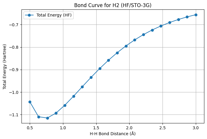
plt.plot(distances, energies, marker='o', label='Total Energy (HF)')
plt.xlabel('H-H Bond Distance (Å)')
plt.ylabel('Total Energy (Hartree)')
plt.title('Bond Curve for H2 (HF/STO-3G)')
plt.grid(True)
plt.legend()
plt.show()
def plot_molecular_orbitals(distances, mo_energies_list):
"""
Plots the molecular orbital energies as a function of bond distance.
Parameters:
- distances (array-like): H-H bond distances.
- mo_energies_list (list of lists): Molecular orbital energies for each distance.
"""
plt.figure(figsize=(8, 5))
for i in range(len(mo_energies_list[0])): # Number of orbitals
orbital_energies = [mo_energies[i] for mo_energies in mo_energies_list]
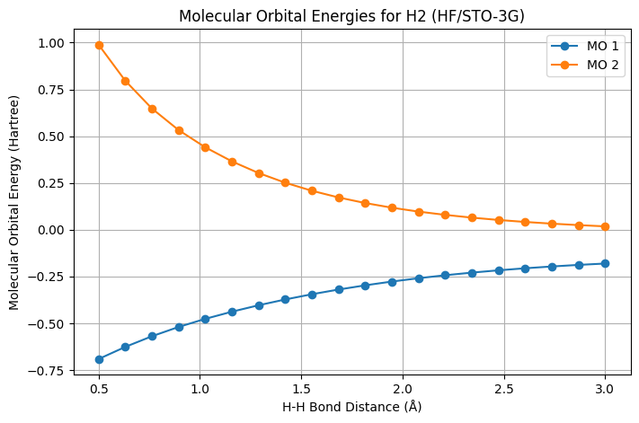
plt.plot(distances, orbital_energies, marker='o', label=f'MO {i+1}')
plt.xlabel('H-H Bond Distance (Å)')
plt.ylabel('Molecular Orbital Energy (Hartree)')
plt.title('Molecular Orbital Energies for H2 (HF/STO-3G)')
plt.grid(True)
plt.legend()
plt.show()
# Define bond distances (in Ångstroms)
distances = np.linspace(0.5, 3.0, 20) # From 0.5 to 3.0 Å
# Run the bond curve calculation
energies, mo_energies_list, mo_coeffs_list = compute_h2_bond_curve(distances)
# Plot the bond curve
plot_bond_curve(distances, energies)
# Plot the molecular orbital energies as a function of bond distance
plot_molecular_orbitals(distances, mo_energies_list)
converged SCF energy = -1.04299627454009
Bond distance: 0.50 Å, Total Energy: -1.042996 Hartree
converged SCF energy = -1.10962287714076
Bond distance: 0.63 Å, Total Energy: -1.109623 Hartree
converged SCF energy = -1.1151049457252
Bond distance: 0.76 Å, Total Energy: -1.115105 Hartree
converged SCF energy = -1.09311721487025
Bond distance: 0.89 Å, Total Energy: -1.093117 Hartree
converged SCF energy = -1.05859984694162
Bond distance: 1.03 Å, Total Energy: -1.058600 Hartree
converged SCF energy = -1.0184750668009
Bond distance: 1.16 Å, Total Energy: -1.018475 Hartree
converged SCF energy = -0.976475042485522
Bond distance: 1.29 Å, Total Energy: -0.976475 Hartree
converged SCF energy = -0.934934347558081
Bond distance: 1.42 Å, Total Energy: -0.934934 Hartree
converged SCF energy = -0.895332352040937
Bond distance: 1.55 Å, Total Energy: -0.895332 Hartree
converged SCF energy = -0.858539335922428
Bond distance: 1.68 Å, Total Energy: -0.858539 Hartree
converged SCF energy = -0.825003227962734
Bond distance: 1.82 Å, Total Energy: -0.825003 Hartree
converged SCF energy = -0.794885434688666
Bond distance: 1.95 Å, Total Energy: -0.794885 Hartree
converged SCF energy = -0.768150987030312
Bond distance: 2.08 Å, Total Energy: -0.768151 Hartree
converged SCF energy = -0.74463276621353
Bond distance: 2.21 Å, Total Energy: -0.744633 Hartree
converged SCF energy = -0.724083718963794
Bond distance: 2.34 Å, Total Energy: -0.724084 Hartree
converged SCF energy = -0.706219811199347
Bond distance: 2.47 Å, Total Energy: -0.706220 Hartree
converged SCF energy = -0.690751272496289
Bond distance: 2.61 Å, Total Energy: -0.690751 Hartree
converged SCF energy = -0.67740092568721
Bond distance: 2.74 Å, Total Energy: -0.677401 Hartree
converged SCF energy = -0.665911797817778
Bond distance: 2.87 Å, Total Energy: -0.665912 Hartree
converged SCF energy = -0.656048251145591
Bond distance: 3.00 Å, Total Energy: -0.656048 Hartree


import numpy as np
from pyscf import gto, scf, tools
import py3Dmol # For 3D visualization of orbitals
def visualize_h2_mo_cubes(bond_distance=0.74, basis='sto-3g', mo_index=0, output_cube_file='mo.cube'):
"""
Generate and visualize cube files for molecular orbitals of H2.
Parameters:
- bond_distance (float): H-H bond distance (in Ångstroms).
- basis (str): Basis set for the calculation (e.g., 'sto-3g', '6-31g').
- mo_index (int): Index of the molecular orbital to visualize (0-indexed).
- output_cube_file (str): The name of the cube file to save.
"""
# 1. Build the H2 molecule
mol = gto.Mole()
mol.atom = f'H 0 0 0; H 0 0 {bond_distance}'
mol.basis = basis
mol.spin = 0 # Singlet state
mol.build()
# 2. Perform Hartree-Fock calculation
mf = scf.RHF(mol)
mf.kernel()
# 3. Generate cube file for the specified molecular orbital (MO)
print(f"Generating cube file for MO {mo_index + 1} (0-indexed as {mo_index})")
tools.cubegen.orbital(mol, output_cube_file, mf.mo_coeff[:, mo_index], nx=80, ny=80, nz=80)
# 4. Visualize the molecular orbital using py3Dmol
print(f"Visualizing cube file: {output_cube_file}")
cube_view = py3Dmol.view(width=400, height=400)
with open(output_cube_file, 'r') as cube_file:
cube_data = cube_file.read()
# Add isosurfaces for positive and negative parts of the orbital
cube_view.addVolumetricData(cube_data, "cube", {'isoval': -0.03, 'color': "red", 'opacity': 0.85})
cube_view.addVolumetricData(cube_data, "cube", {'isoval': 0.03, 'color': "blue", 'opacity': 0.85})
# Add the molecular structure as well
cube_view.addModel(mol.tostring(format="xyz"), 'xyz')
cube_view.setStyle({'stick': {}, 'sphere': {'radius': 0.4}})
cube_view.setBackgroundColor('0xeeeeee')
cube_view.show()
# Set the bond distance, basis, and the index of the molecular orbital to visualize
visualize_h2_mo_cubes(bond_distance=0.74, basis='sto-3g', mo_index=1, output_cube_file='mo_1.cube') # MO 1
converged SCF energy = -1.11675930739643
Generating cube file for MO 2 (0-indexed as 1)
Visualizing cube file: mo_1.cube
3Dmol.js failed to load for some reason. Please check your browser console for error messages.

