Linear Algebra 1: Basics

Linear Algebra 1: Basics#

Vectors, what are they?#

../_images/0256d990cafb4436aa04a235573ffb51bd38e00dd7238db675010ffab608fbce.png

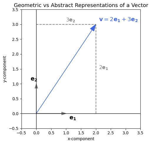
Abstract Representations:

$$ \mathbf{v} = \begin{pmatrix} 2 \ 3 \end{pmatrix} \quad \Longleftrightarrow \quad |v\rangle = 2|e_1\rangle + 3|e_2\rangle $$

Vectors as Arrays of Numbers#

A vector is an ordered collection of numbers that represents the state or configuration of a physical system.

$a = (-2, 8)$ — a 2D vector
$e_1$ = (1,0) - a unit vector along x axis and $e_2 = (0,1)$ a unit vector along y axis
$b = (1.34, 4.23, 5.98)$ — a 3D vector
$c = (1, -2, 4i, 3 + 2i)$ — a 4D vector with complex components
$f = (1, 2, 3, 4, 5, 6, \ldots)$ — an infinite-dimensional vector (e.g., a sequence)

Note: Vectors may belong to real or complex vector spaces depending on the nature of their components.

Vector Space

Any vector in an $N$-dimensional space can be written as a linear combination of $N$ linearly independent basis vectors.
For instance, in 2D space, we can choose two perpendicular unit vectors $e_1$ and $e_2$ to form a convenient basis:

\[\begin{split} \vec{a} = a_1 e_1 + a_2 e_2 = \begin{pmatrix} a_1\\ a_2\\ \end{pmatrix} \end{split}\]

\[\begin{split}a= \begin{pmatrix} 2\\ 3\\ \end{pmatrix} = 2\begin{pmatrix} 1\\ 0\\ \end{pmatrix}+3 \begin{pmatrix} 0\\ 1\\ \end{pmatrix} \end{split}\]

If we choose a rotated basis $e'_1$, $e'_2$ (e.g choose basis vectors with length 2), the components change, but the vector itself remains the same:

\[ \vec{a} = a'_1 e'_1 + a'_2 e'_2 = (a'_1, a'_2) \]

\[\begin{split}a= \begin{pmatrix} 2\\ 3\\ \end{pmatrix} = 1\begin{pmatrix} 2\\ 0\\ \end{pmatrix}+\frac{3}{2} \begin{pmatrix} 0\\ 2\\ \end{pmatrix} \end{split}\]

Row and Column Vectors#

In linear algebra and quantum mechanics, we distinguish between column vectors (kets) and row vectors (bras), which are related by the transpose (and, in complex spaces, by the Hermitian conjugate):

\[ \langle a | = \begin{pmatrix} a_1 \ a_2 \end{pmatrix} \]

\[\begin{split} |b\rangle = \begin{pmatrix} b_1\\ b_2\\ \end{pmatrix} \end{split}\]

Although they describe the same state or object, bras and kets “live” in dual spaces — column vectors form one space, while row vectors belong to its dual space. Their interaction through the inner product $\langle b | a \rangle$ gives a scalar quantity.

Inner products and orthogonality#

Dot product $\langle a\mid b \rangle$ quantifies the projection of vector $a$ on $b$ and vice-versa. That is, how much $a$ and $b$ have in common in terms of direction in space!

Dot product: geometric definition

\[ \langle a\mid b \rangle = |a| |b| cos\theta \]

The $\theta$ measures angle between a and b. If vectors are perpendicular like unit vectors in cartesian system we call them orthogonal
Orthonormal vectors are both normalized and orthogonal. We denote orthornamilty condition with the convenient Kornecker symbol: $\delta_{ij}=0$ when $i\neq j$ and $1$ when $i=j$.

\[ \langle e_i \mid e_j \rangle =\delta_{ij} \]

\[\begin{split} (1,0)\begin{pmatrix} 0\\ 1\\ \end{pmatrix}=1\cdot 0+0\cdot 1=0 \end{split}\]

Norm of a vector $\mid a\mid$ Is project of the vector onto itself and quantifies the length of the vector. When the norm is $\mid a \mid=1$, we say that the vector is normalized.

\[ \langle a \mid a\rangle= \big(a_1\langle e_1| + a_2 \langle e_2|\big) \cdot \big (a_1 |e_1\rangle + a_2 |e_2 \rangle \big ) = a_1^2+a_2^2 \]

\[ \mid a \mid =\sqrt{a_1^2+a_2^2} \]

Inner product between two vectors

\[\vec{a} \cdot \vec{b} = \langle a| b \rangle = a_1 b_1+ a_2b_2+ ... \]

Use inner product to defiine components

\[\vec{a_1} = a_1 e_1 + a_2 \vec{e}_2+ ...\]

\[\vec{e_1} \cdot \vec{a} = a_1\]

\[\langle e_1 | a_1\rangle = a_1\]

Decomposition of functions into orthogonal components#

Writing a vector in terms of its orthogonal unit vectors is a powerful mathematical technique which permeates much of quantum mechanics. The role of finite dimensional vectors in QM play the infinite dimensional functions. In analogy with sequence vectors which can live in 2D, 3D or ND spaces, the inifinite dimensional space of functions in quantum mathematics is known as a Hilbert space, named after famous mathematician David Hilbert. We will not go too much in depth about functional spaces other than listing some powerful analogies with simple sequence vectors.

Vectors	Functions
Orthonormality $\\ \langle x\mid y \rangle = \sum^{i=N}_{i=1} x_i y_i=\delta_{xy}$	Orthonormality $\\ \langle \phi_i \mid \phi_j \rangle = \int^{+\infty}_{-\infty} \phi_i(x) \phi_j(x)dx=\delta_{ij}$
Linear superposition $\\ \mid A \rangle = A_x \mid x\rangle+A_y\mid y\rangle$	Linear superposition $\\ \mid f\rangle = c_1 \mid\phi_1\rangle+c_2\mid\phi_2\rangle$
Projections $\\ \langle e_x\mid A\rangle=A_x \langle x\mid x \rangle +A_y \langle x\mid y \rangle=A_x $	Projections $\\ \langle \phi_1\mid \Psi\rangle=c_1 \langle \Psi \mid\phi_1 \rangle +c_2 \langle \Psi \mid\phi_2 \rangle=c_1$

System of Linear Equations as Matrix Operations#

A system of linear equations can be interpreted as a matrix operating on a vector to produce another vector. For example, consider the system:

\[\begin{split} \begin{aligned} a_{11}x_1 + a_{12}x_2 &= b_1 \\ a_{21}x_1 + a_{22}x_2 &= b_2 \end{aligned} \end{split}\]

This system can be written compactly in matrix form as:

A system of linear equation as matrix vector product

\[ A \mathbf{x} = \mathbf{b} \]

$A$ is a matrix containing the coefficients of the system,
$\mathbf{x}$ is the vector of unknowns, and
$\mathbf{b}$ is the vector of constants (right-hand side).

For a 2D system, this becomes:

\[\begin{split} \begin{pmatrix} a_{11} & a_{12} \\ a_{21} & a_{22} \end{pmatrix} \begin{pmatrix} x_1 \\ x_2 \end{pmatrix} = \begin{pmatrix} b_1 \\ b_2 \end{pmatrix} \end{split}\]

Matrix vector Multiplication#

Row by column product rule

Matrix multiplication operates by taking the dot product of the rows of the matrix $A$ with the vector $\mathbf{x}$. For the above example:

\[\begin{split}A \mathbf{x} = \begin{pmatrix} a_{11}x_1 + a_{12}x_2 \\ a_{21}x_1 + a_{22}x_2 \end{pmatrix} \end{split}\]

This shows how the system of equations is equivalent to multiplying the matrix by the vector.

Lower level definition of Matrix Multiplication

In general, if $A$ is an $m \times n$ matrix and $\mathbf{x}$ is a vector of dimension $n$, the matrix-vector multiplication $A \mathbf{x}$ is defined as:

\[ b_i = (A \mathbf{x})_i = \sum_{j=1}^{n} a_{ij} x_j \]

Where $a_{ij}$ are the elements of matrix $A$, and $x_j$ are the components of vector $\mathbf{x}$.

Solving linear equation via matrix Inversion

\[{\bf x} = A^{-1}{\bf b}\]

Solving Ax=b via matrix inversion
A [[ 2  3]
 [ 1 -2]]
b [7 1]
Solution using matrix inversion:
x = [2.42857143 0.71428571]

Eigenvalues and Eigenvectors#

When a matrix acts on a vector, it generally changes both its direction and length. However, there are special vectors that preserve their direction—they are only scaled by the transformation. These are called eigenvectors, and the corresponding scaling factors are eigenvalues.

Definition of Eigenvalue Problem

A vector $\mathbf{v}$ is an eigenvector of a matrix $A$ if

\[ A \mathbf{v} = \lambda \mathbf{v}, \]

where $\lambda$ is a scalar called the eigenvalue.

In this equation:

$A$ is the linear transformation (matrix or operator),
$\mathbf{v}$ is a non-zero vector whose direction remains unchanged,
$\lambda$ tells how much $\mathbf{v}$ is stretched, compressed, or flipped.

Finding Eigenvalues#

Rearranging the equation gives:

\[ (A - \lambda I)\mathbf{v} = 0. \]

For a nontrivial solution ($\mathbf{v} \neq 0$), the determinant must vanish:

\[ \det(A - \lambda I) = 0. \]

This condition is the characteristic equation of the matrix and yields the possible eigenvalues $\lambda$.

Geometric Meaning#

If $\lambda > 1$: the vector is stretched.
If $0 < \lambda < 1$: the vector is compressed.
If $\lambda < 0$: the vector is flipped in direction.
If $\lambda = 0$: the vector is collapsed to the origin.

In quantum mechanics, this idea generalizes to operators acting on wavefunctions—where eigenvalues correspond to measurable quantities (observables) and eigenvectors to the states with definite outcomes.

Property	Expression	Meaning
Eigenvalue equation	$A\mathbf{v} = \lambda\mathbf{v}$	Defines scaling along eigenvector
Inverse action	$A^{-1}\mathbf{v} = \frac{1}{\lambda}\mathbf{v}$	Inverse rescales in opposite way
Invertibility condition	$\det(A) \neq 0$ or all $\lambda \neq 0$	Matrix is invertible only if no eigenvalue is zero

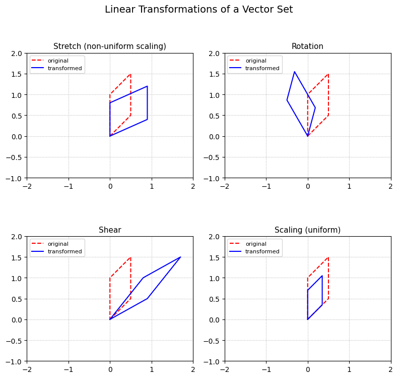
Visualizing Action of a Matrix on a Vector#

These transformations illustrate different ways of modifying vectors and geometric shapes through scaling, shearing, and identity operations. We use a 2D vector and matrices as an example.

Matrix Type	Example	Effect
Diagonal, unequal entries	`[[2, 0], [0, 0.5]]`	Stretch — different scaling per axis
Diagonal, equal entries	`[[0.7, 0], [0, 0.7]]`	Uniform scaling — isotropic compression
Orthogonal (rotation matrix)	`[[cosθ, -sinθ], [sinθ, cosθ]]`	Rotation — preserves lengths and angles
Off-diagonal elements	`[[1, k], [0, 1]]`	Shear — slants axes without changing area

We pick the folloing four dummy vectors and act our matrix on all of them to see how the relationship between their distances and angles changes

\[(0,0), (0.5,0.5), (0.5, 1.5), (0,1), (0,0)\]

We connect the points defined by this vectors to aid our visualization

../_images/db52373bb1dc039d346c2bdbbbe5282b9a1fe61ba6196b815a7be0e70f88cca8.png

Vectors	Functions
Orthonormality \(\\ \langle x\mid y \rangle = \sum^{i=N}_{i=1} x_i y_i=\delta_{xy}\)	Orthonormality \(\\ \langle \phi_i \mid \phi_j \rangle = \int^{+\infty}_{-\infty} \phi_i(x) \phi_j(x)dx=\delta_{ij}\)
Linear superposition \(\\ \mid A \rangle = A_x \mid x\rangle+A_y\mid y\rangle\)	Linear superposition \(\\ \mid f\rangle = c_1 \mid\phi_1\rangle+c_2\mid\phi_2\rangle\)
Projections \(\\ \langle e_x\mid A\rangle=A_x \langle x\mid x \rangle +A_y \langle x\mid y \rangle=A_x \)	Projections \(\\ \langle \phi_1\mid \Psi\rangle=c_1 \langle \Psi \mid\phi_1 \rangle +c_2 \langle \Psi \mid\phi_2 \rangle=c_1\)

Property	Expression	Meaning
Eigenvalue equation	\(A\mathbf{v} = \lambda\mathbf{v}\)	Defines scaling along eigenvector
Inverse action	\(A^{-1}\mathbf{v} = \frac{1}{\lambda}\mathbf{v}\)	Inverse rescales in opposite way
Invertibility condition	\(\det(A) \neq 0\) or all \(\lambda \neq 0\)	Matrix is invertible only if no eigenvalue is zero