Particle in a Box

What you need to know

Particle in a Box (PIB) as a Model System
The Particle in a Box (PIB) is a simple model that helps illustrate the behavior of electrons confined within atoms and molecules. It serves as a useful tool to introduce key quantum concepts:

• Energetic Quantization: Energy levels in quantum systems are discrete, not continuous, as seen in the PIB model.

• Probabilistic Nature of Quantum Particles: The probability distribution for the particle’s position is non-uniform, with nodal points where the probability is zero, emphasizing the inherent uncertainty in the particle’s exact location.

• Uncertainty Principle: There is an inverse relationship between the uncertainty in position and momentum, demonstrating the fundamental limit on how precisely both quantities can be known simultaneously.

• Zero-Point Energy: Quantum particles always possess a minimum kinetic energy, even at absolute zero. This zero-point energy highlights the impossibility of freezing all motion in quantum systems.

• Quantum-Classical Correspondence: As the system scales up, quantum behavior smoothly transitions to classical behavior, illustrating the correspondence principle.

• Degeneracy of Energy Levels: In systems with symmetries, multiple wave functions can correspond to the same energy level, a phenomenon known as degeneracy.

Classical vs Quantum particle in a box

• Particle in a box is a toy model of electron (or atom, molecule, small quantum object) trapped in some region of space \([0,L]\).

• The positional information of a quantum “particle” is described by a quantum wave function \(\psi(x)\) which is obtained by solving Schrödinger equation with boundary conditions

• Wave functions are standing waves just like in a guitar on a string problem. With one major difference! Quantum-wave function has a probabilistic meaning and hence has a completely different meaning from a classical notion of a “wave”.

• According to classical mechanis in the absence of any attractive interactions particle will be boundicng back and forth between walls with constant speed. Hence and we expect to find particle with equal probability at all locations \(x\).

• According to quantum mechancis Quantum particle in the box is going to be found in some regions with high probability in others with little or zero!

Fig. 51 The particle in a box (PIB) is a convenient system for illustrating the differences between classical (A) and quantum systems (B-F). The horizontal axis is position, and the vertical axis is the real part (blue) and imaginary part (red) of the wavefunction \(\psi_n(x)\). The states (B,C,D) are the eigenfunctions of Hamiltonian \(n=1,2,3\). While E and F are not.

Solving the Schrödinger Equation for the Particle in a Box (PIB)

Fig. 52 Particle in a box subject to infinitely high potential walls

The Schrödinger equation for a particle in a box (PIB) is defined by a Hamiltonian operator that incorporates the potential energy, which is infinitely large at the boundaries of the box and zero inside. This potential ensures that the particle is confined within the box, where it can only possess kinetic energy.

• The potential energy for PIB is defined:

\[\begin{split} V(x) = \begin{cases} \infty & x = 0 \text{ or } x = L \\ 0 & 0 < x < L \end{cases} \end{split}\]

• The boundary conditions are:

\[ \psi(0) = \psi(L) = 0 \]

• The Hamiltonian operator is in this case accounting only for kinetic energy!

\[ \hat{H} = \hat{K} = -\frac{\hbar^2}{2m} \frac{d^2}{dx^2} \]

• Now, we have all the necessary ingredients to solve the time-independent Schrödinger equation for the 1D PIB:

\[ \hat{H} \psi(x) = E \psi(x) \]

• Substituting the Hamiltonian, we get:

\[ -\frac{\hbar^2}{2m} \frac{d^2}{dx^2} \psi(x) = E \psi(x) \]

\[ \psi''(x) = -k^2 \psi(x) \]

• where the \(k^2\) is a positive real number that relates the particle’s energy \(E\) to its wavefunction.

\[ k^2 = \frac{2mE}{\hbar^2} \]

Solution and Boundary Conditions

• Mathematically, the form of the 1D PIB problem is similar to the ordinary differential equation (ODE) used in the 1D vibrating guitar string problem. The key differences lie in the constant coefficients and the interpretation of the wavefunction.

\[ \psi''(x) = -k^2 \psi(x) \]

• The general solution to this differential equation is:

\[ \psi(x) = c_1 e^{ikx} + c_2 e^{-ikx} = A \cos(kx) + B \sin(kx) \]

• Applying the boundary condition \(\psi(0) = 0\), we find that \(A = 0\), leaving us with:

\[ \psi(x) = B \sin(kx) \]

• Applying the boundary condition \(\psi(L) = 0\), we get:

\[ B \sin(kL) = 0 \]

• This condition is satisfied when:

\[ kL = n\pi \quad \text{or} \quad k = \frac{n\pi}{L} \]

• Thus, the wavefunction becomes:

\[ \psi(x) = B \sin\left(\frac{n\pi}{L}x\right) \]

• Using the relationship \(k^2 = \frac{n^2\pi^2}{L^2} = \frac{2mE}{\hbar^2}\), we can express the energy levels as:

\[ E_n = \frac{n^2 h^2}{8mL^2} \]

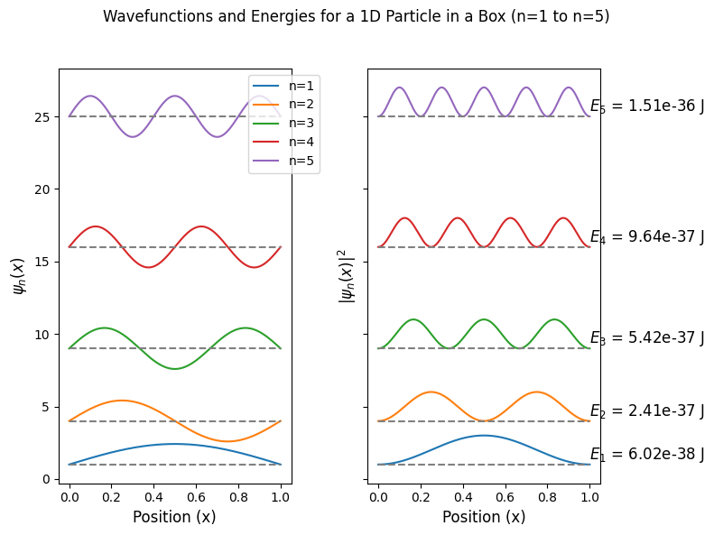
• The quantization of energy results from confining the wavefunction within a finite space. This is the reason bound states exhibit quantized energy levels. Atoms, molecules, and solids all possess discrete energy levels due to similar constraints.

Wavefunctions Must Be Normalized

• Next, we determine the constant coefficient \(B_n\) by enforcing the normalization condition:

\[ \int_0^L \psi_n(x)^2 \, dx = 1\]

• To evaluate the integral, we use the trigonometric identity \(\sin^2(x) = \frac{1}{2}(1 - \cos(2x))=1\)

\[ B_n^2 \int_0^L \sin^2\left(\frac{n\pi x}{L}\right) dx = \frac{B_n^2}{2} \int_0^L \left[ 1 - \cos\left(\frac{2n\pi x}{L}\right) \right] dx =1 \]

• Since the integral of \(\cos\left(\frac{2n\pi x}{L}\right)\) over a full period from \(0\) to \(L\) is zero, we are left with:

\[ \frac{B_n^2}{2} \cdot L = 1 \]

• Solving for \(B_n\) we determine normalization constant which ensures that square of wavefunction integrates to 1.

\[ B_n = \sqrt{\frac{2}{L}} \]

PIB Eigenfunctions and Eigenvalues

Eigenfunctions and eigenvalues of 1D particle in a box

\[{\psi_n(x) = \Big (\frac{2}{L}\Big)^{\frac{1}{2}} \sin\frac{n\pi x}{L}}\]

\[{E_n=\frac{n^2 h^2}{8mL^2}}\]

Full time dependent solution

\[{\psi_n(x, t) = \Big (\frac{2}{L}\Big)^{\frac{1}{2}} \sin\frac{n\pi x}{L}}\cdot e^{-i\frac{E_n t}{\hbar}}\]

\[\Psi(x,t) = \sum_n c_n \psi_n(x, t)\]

• Where the coefficients \(c_n\) depend on initial condition, e.g could be all zero except one (pure state) or a few of them non-zero (mixed state)

Show code cell source Hide code cell source

import numpy as np
import matplotlib.pyplot as plt

# Parameters
L = 1.0  # Length of the box
x = np.linspace(0, L, 1000)  # Position array
n_max = 5  # Maximum quantum number to display

# Constants
hbar = 1.0545718e-34  # Reduced Planck's constant (J·s)
m = 9.10938356e-31  # Mass of an electron (kg)

# Functions
def psi_n(n, x, L):
    """Wavefunction for a particle in a 1D box."""
    return np.sqrt(2 / L) * np.sin(n * np.pi * x / L)

def psi_n_squared(n, x, L):
    """Probability density (wavefunction squared)."""
    return psi_n(n, x, L) ** 2

def energy_levels(n, L):
    """Energy level for the particle in the box."""
    return (n**2 * np.pi**2 * hbar**2) / (2 * m * L**2)

# Energy formula string
energy_formula = r"$E_n = \frac{n^2 \pi^2 \hbar^2}{2mL^2}$"

# Plotting
fig, axs = plt.subplots(1, 2, figsize=(8, 6), sharey=True)

# Plot wavefunctions in the first subplot
for n in range(1, n_max + 1):
    wavefunction = psi_n(n, x, L)
    axs[0].plot(x, wavefunction + n**2, label=f'n={n}')
    axs[0].hlines(n**2, 0, L, colors='gray', linestyles='dashed')  # Energy level lines

# Wavefunction plot labels and title
axs[0].set_xlabel('Position (x)', fontsize=12)
axs[0].set_ylabel(r'$\psi_n(x)$', fontsize=12)
axs[0].legend(loc='upper right', bbox_to_anchor=(1.15, 1))

# Plot wavefunction squared (probability densities) in the second subplot
for n in range(1, n_max + 1):
    wavefunction_squared = psi_n_squared(n, x, L)
    axs[1].plot(x, wavefunction_squared + n**2, label=f'n={n}')
    axs[1].hlines(n**2, 0, L, colors='gray', linestyles='dashed')  # Energy level lines

# Probability density plot labels
axs[1].set_xlabel('Position (x)', fontsize=12)
axs[1].set_ylabel(r'$|\psi_n(x)|^2$', fontsize=12)

# Display the energy formula and levels in the second subplot
for n in range(1, n_max + 1):
    energy_value = energy_levels(n, L)
    axs[1].text(L, n**2, f"$E_{n}$ = {energy_value:.2e} J", verticalalignment='bottom', fontsize=12)

# Overall title for the figure
fig.suptitle(f'Wavefunctions and Energies for a 1D Particle in a Box (n=1 to n={n_max})')

# Make room for labels outside plot and improve layout
plt.tight_layout(rect=[0, 0, 1, 0.95])
plt.show()

Discrete energy levels and zero point energy

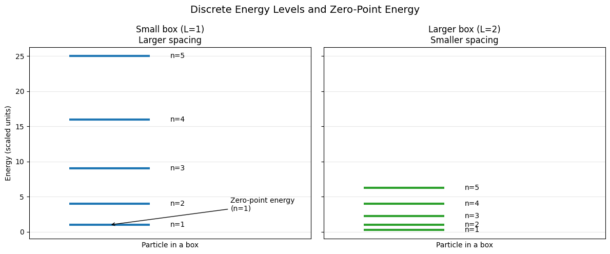
Quantum particles are never at rest

• The lowest energy electon in a box can have is at \(n=1\) at which is not zero!

\[E_1 = h^2/8mL^2\]

• Keeping in mind that the energy is purely kinetic, this means quantum particles never ceases their motion.

• The spacing of energy levels is finite and depends on the size of the box!

\[E_{n+1} - E_n = (2n+1)\frac{h^2}{8mL^2}\]

Increasing Box size leads to more classical behavior

• As the box size is increased energy spacing gets smaller!

• Thus quantum effects are more pronounced when electorn is bound in smaller regions of space.

Non-uniform probabilities and nodes

• There are \(n-1\) nodes for quantum state \(n\)

• Recall that sine function hitz zero at integer values of \(\pi\), \(sin(n\pi)=0\) when \(n=1,2,3,4,...\)

• The wavefunction \(\psi_n(x) = sin \frac{n\pi x}{L}\) will then have \(n-1\) nodes at points \(x=L/n\), \(2L/n\), \(3L/n\), … \((n-1)L/n\).

• Note that we do not count \(x=0\) and \(x=L\) points as nodes because they are part of boudnary conditions that apply to all wavefunctions

  • For instance \(n=3\) nodes are at \(x=L/3\), \(x=2L/3\).

  • For instance \(n=4\) nodes are at \(L/4\), \(2L/4\), \(3L/4\)

• Nodes imply zero probability to find an electron in the box.

  • \(|\psi_n|^2=0\) at nodal points which means zero probability.

  • This is in sharp contradiction of classical mechanics which bases its prediction on purely particle like motion of electron.

  • Existence of nodes implies a wave like character of electron

On time-dependence

Pure states

• Pure states correspond to time-independent probability distribution.

\[|\psi_n(x,t)|^2 = \psi_n(x,t)^{*}\cdot\psi_n(x,t) = \psi(x)e^{-iE_nt/\hbar}\cdot \psi(x)e^{+E_nt/\hbar} = |\psi(x)|^2\]

• Below we visualize a few of the wavefunction at its square for \(n=2\).

Show code cell source Hide code cell source

import numpy as np
import matplotlib.pyplot as plt
from matplotlib.animation import FuncAnimation
from IPython.display import HTML

# Parameters
L = 1.0  # Length of the box
hbar = 1.0  # Set hbar = 1 for simplicity
m = 1.0  # Set mass = 1 for simplicity

# Define spatial and time arrays
x = np.linspace(0, L,  200)  
t = np.linspace(0, 10, 200)  

n = 2

# Define energy for nth state
def energy_n(n, L):
    return (n**2 * np.pi**2 * hbar**2) / (2 * m * L**2)

# Define wavefunction for nth state
def psi_total(n, x, L, t):
    E_n = energy_n(n, L)
    return np.sqrt(2 / L) * np.sin(n * np.pi * x / L) * np.exp(-1j * E_n * t / hbar)


# Set up the figure and axis
fig, (ax1, ax2) = plt.subplots(1, 2, figsize=(11, 8))

# Set limits for the wavefunction and wavefunction squared
ax1.set_xlim(0, L)
ax1.set_ylim(-2, 2)
ax2.set_xlim(0, L)
ax2.set_ylim(0, 4)

# Set labels for the wavefunction plot
ax1.set_xlabel('Position (x)', fontsize=14)
ax1.set_ylabel(r'Re[$\psi(x,t)$]', fontsize=14)
ax1.set_title('Time Evolution of Wavefunction', fontsize=16)

# Set labels for the squared wavefunction plot
ax2.set_xlabel('Position (x)', fontsize=14)
ax2.set_ylabel(r'$|\psi(x,t)|^2$', fontsize=14)
ax2.set_title('Probability Density', fontsize=16)

### Animation settings 

# Initialize the wavefunction and its square plots
line_real, = ax1.plot([], [], lw=2)
line_prob, = ax2.plot([], [], lw=2)

# Initialization function for the plot
def init():
    line_real.set_data([], [])
    line_prob.set_data([], [])
    return line_real, line_prob

# Animation function which updates the plot each frame
def animate(i):
    t_val = t[i]
    psi = psi_total(n, x, L, t_val)
    psi_real = np.real(psi)
    psi_squared = np.abs(psi)**2
    line_real.set_data(x, psi_real)
    line_prob.set_data(x, psi_squared)
    return line_real, line_prob

# Create the animation
ani = FuncAnimation(fig, animate, init_func=init, frames=len(t), interval=150, blit=True)

plt.close(fig)  # Prevents static display of the last frame
HTML(ani.to_jshtml())

Once Loop Reflect

Mixed states

• Mixed states show time dependence. Below we visualize lienar combination of the first two eigenfunctions of PIB.

\[ \psi(x,t) = c_1 \psi_1(x) e^{-iE_1t/\hbar} +c_2 \psi_2 e^{-iE_2t/\hbar} \]

Step-by-Step illustration of time-dependence

1. The complex conjugate of \(\psi(x,t)\) is:

\[ \psi^*(x,t) = c_1^* \psi_1(x) e^{iE_1t/\hbar} + c_2^* \psi_2(x) e^{iE_2t/\hbar} \]

2. The squared wavefunction \(|\psi(x,t)|^2\) is:

\[ |\psi(x,t)|^2 = \left( c_1 \psi_1(x) e^{-iE_1t/\hbar} + c_2 \psi_2(x) e^{-iE_2t/\hbar} \right) \left( c_1^* \psi_1(x) e^{iE_1t/\hbar} + c_2^* \psi_2(x) e^{iE_2t/\hbar} \right) \]

3. Expanding the product:

\[ |\psi(x,t)|^2 = |c_1|^2 |\psi_1(x)|^2 + |c_2|^2 |\psi_2(x)|^2 + c_1 c_2^* \psi_1(x) \psi_2^*(x) e^{-i(E_1 - E_2)t/\hbar} + c_1^* c_2 \psi_1^*(x) \psi_2(x) e^{i(E_1 - E_2)t/\hbar} \]

Final Expression

\[ |\psi(x,t)|^2 = |c_1|^2 |\psi_1(x)|^2 + |c_2|^2 |\psi_2(x)|^2 + 2 \, \text{Re} \left[ c_1 c_2^* \psi_1(x) \psi_2^*(x) e^{-i(E_1 - E_2)t/\hbar} \right] \]

This consists of:

• The probability densities of \(\psi_1(x)\) and \(\psi_2(x)\) with coefficients \(|c_1|^2\) and \(|c_2|^2\).

• A time-dependent interference term that oscillates with the frequency \((E_1 - E_2)/\hbar\).

Show code cell source Hide code cell source

import numpy as np
import matplotlib.pyplot as plt
from matplotlib.animation import FuncAnimation
from IPython.display import HTML

# Parameters
L = 1.0  # Length of the box
hbar = 1.0  # Set hbar = 1 for simplicity
m = 1.0  # Set mass = 1 for simplicity

n_states = [1, 2]  # Quantum numbers for the superposition
coeffs = [1, 1]  # Coefficients for the superposition
coeffs = np.array(coeffs) / np.sqrt(np.sum(np.array(coeffs) ** 2))  # Normalize coefficients

# Define spatial and time arrays
x = np.linspace(0, L,  200)  
t = np.linspace(0, 10, 200)  

# Define wavefunction for nth state
def psi_n(n, x, L):
    return np.sqrt(2 / L) * np.sin(n * np.pi * x / L)

# Define energy for nth state
def energy_n(n, L):
    return (n**2 * np.pi**2 * hbar**2) / (2 * m * L**2)

# Define time-dependent wavefunction
def psi_total(x, t, L, coeffs, n_states):
    psi_t = np.zeros_like(x, dtype=complex)
    for idx, n in enumerate(n_states):
        psi_x = psi_n(n, x, L)
        E_n = energy_n(n, L)
        time_factor = np.exp(-1j * E_n * t / hbar)
        psi_t += coeffs[idx] * psi_x * time_factor
    return psi_t

# Set up the figure and axis
fig, (ax1, ax2) = plt.subplots(1, 2, figsize=(11, 8))

# Set limits for the wavefunction and wavefunction squared
ax1.set_xlim(0, L)
ax1.set_ylim(-2, 2)
ax2.set_xlim(0, L)
ax2.set_ylim(0, 4)

# Set labels for the wavefunction plot
ax1.set_xlabel('Position (x)', fontsize=14)
ax1.set_ylabel(r'Re[$\psi(x,t)$]', fontsize=14)
ax1.set_title('Time Evolution of Wavefunction', fontsize=16)

# Set labels for the squared wavefunction plot
ax2.set_xlabel('Position (x)', fontsize=14)
ax2.set_ylabel(r'$|\psi(x,t)|^2$', fontsize=14)
ax2.set_title('Probability Density', fontsize=16)

### Animation settings 

# Initialize the wavefunction and its square plots
line_real, = ax1.plot([], [], lw=2)
line_prob, = ax2.plot([], [], lw=2)

# Initialization function for the plot
def init():
    line_real.set_data([], [])
    line_prob.set_data([], [])
    return line_real, line_prob

# Animation function which updates the plot each frame
def animate(i):
    t_val = t[i]
    psi = psi_total(x, t_val, L, coeffs, n_states)
    psi_real = np.real(psi)
    psi_squared = np.abs(psi)**2
    line_real.set_data(x, psi_real)
    line_prob.set_data(x, psi_squared)
    return line_real, line_prob

# Create the animation
ani = FuncAnimation(fig, animate, init_func=init, frames=len(t), interval=150, blit=True)

plt.close(fig)  # Prevents static display of the last frame
HTML(ani.to_jshtml())

Once Loop Reflect

Quantum PIB in 3D

Fig. 53 Particle in a 3D box subject to infinitely high potential walls.

\[\hat{H}\psi(x,y,z) = E\psi(x,y,z)\]

\[{-\frac{\hbar^2}{2m}\left(\frac{\partial^2\psi}{\partial x^2} + \frac{\partial^2\psi}{\partial y^2} + \frac{\partial^2\psi}{\partial z^2}\right) = E\psi}\]

• Where we set \(V=0\) for particle inside the box and enforce the solutions \(\psi\) to be normalized within the confines of the box (electron must be somewhere in the box!)

\[{\int\limits_{-\infty}^{\infty}\int\limits_{-\infty}^{\infty}\int\limits_{-\infty}^{\infty}\left|\psi(x,y,z)\right|^2dxdydz = 1}\]

• Consider a particle in a box with sides of lengths \(a\) in \(x\), \(b\) in \(y\) and \(c\) in \(z\). The potential inside the box is zero and outside the box infinity. Again, the potential term can be treated by boundary conditions (i.e,. infinite potential implies that the wavefunction must be zero there). The above equation can be now written as:

\[\begin{split}{-\frac{\hbar^2}{2m}\Delta\psi = E\psi} \\ {\textnormal{with }\psi(a,y,z) = \psi(x,b,z) = \psi(x,y,c) = 0} \\ {\textnormal{and }\psi(0,y,z) = \psi(x,0,z) = \psi(x,y,0) = 0}\end{split}\]

• Note the nabla symbol \(\Delta\) which concisely denotes the sum of three second order derivatives with respect to spatial variables. We will see this operators in all 3D problems.

• In general, when the potential term can be expressed as a sum of terms that depend separately only on \(x, y\) and \(z\), the solutions can be written as a product:

\[{\psi(x,y,z) = X(x)Y(y)Z(z)}\]

• By substituting and dividing by \(X(x)Y(y)Z(z)\), we obtain:

\[{-\frac{\hbar^2}{2m}\left[\frac{1}{X(x)}\frac{d^2X(x)}{dx^2} + \frac{1}{Y(y)}\frac{d^2Y(y)}{dy^2} + \frac{1}{Z(z)}\frac{d^2Z(z)}{dz^2}\right] = E}\]

• The total energy \(E\) consists of a sum of three terms. Each tersm depends separately on \(x, y\) and \(z\). Thus we can write \(E = E_x + E_y + E_z\) and separate the equation into three one-dimensional problems.

\[\begin{split}{-\frac{\hbar^2}{2m}\left[\frac{1}{X(x)}\frac{d^2X(x)}{dx^2}\right] = E_x\textnormal{ with }X(0) = X(a) = 0}\\ {-\frac{\hbar^2}{2m}\left[\frac{1}{Y(y)}\frac{d^2Y(y)}{dy^2}\right] = E_y\textnormal{ with }Y(0) = Y(b) = 0}\\ {-\frac{\hbar^2}{2m}\left[\frac{1}{Z(z)}\frac{d^2Z(z)}{dz^2}\right] = E_z\textnormal{ with }Z(0) = Z(c) = 0}\end{split}\]

• Thus we find that energy quantization due to spatial confinement of quantum wave function in X, Y and Z dimensions.

\[\begin{split}{X(x) = \sqrt{\frac{2}{a}}\sin\left(\frac{n_x\pi x}{a}\right)}\\ {Y(y) = \sqrt{\frac{2}{b}}\sin\left(\frac{n_y\pi y}{b}\right)}\\ {Z(z) = \sqrt{\frac{2}{c}}\sin\left(\frac{n_z\pi z}{c}\right)}\end{split}\]

Non-cubic Box

\[{\psi(x,y,z) = X(x)Y(y)Z(z) = \sqrt{\frac{8}{abc}}\sin\left(\frac{n_x\pi x}{a}\right)\sin\left(\frac{n_y\pi y}{b}\right)\sin\left(\frac{n_z\pi z}{c}\right)}\]

\[{E_{n_x,n_y,n_z} = \frac{h^2}{8m}\left(\frac{n_x^2}{a^2} + \frac{n_y^2}{b^2} + \frac{n_z^2}{c^2}\right)}\]

Eigenfunctions and eigenvalues of particle in 3D Box

Cubix Box

\[ \psi_{n_x, n_y, n_z}(x, y, z) = \frac{2}{L^{3/2}} \sin\left( \frac{n_x \pi x}{L} \right) \sin\left( \frac{n_y \pi y}{L} \right) \sin\left( \frac{n_z \pi z}{L} \right) \]

\[ E_{n_x, n_y, n_z} = \frac{\hbar^2 \pi^2}{2mL^2} \left( n_x^2 + n_y^2 + n_z^2 \right) \]

• Energy is quantized and when \(a = b = c\), we find that the energy levels can also be degenerate (i.e., the same energy with different values of \(n_x, n_y\) and \(n_z\)).

• In most cases, degeneracy in quantum mechanics arises from symmetry. When \(a = b = c\), the lowest levels have the following degeneracy factors:

Table of energy levels for 3D box

Quantum Numbers \(( n_x, n_y, n_z\))	Energy \(( E_{n_x, n_y, n_z} )\)	Degeneracy
(1,1,1)	\(( \frac{3\hbar^2}{2mL^2} ) \)	1
(1,1,2), (1,2,1), (2,1,1)	\(( \frac{6\hbar^2}{2mL^2} ) \)	3
(1,1,3), (1,3,1), (3,1,1)	\(( \frac{11\hbar^2}{2mL^2} ) \)	3
(1,2,2), (2,1,2), (2,2,1)	\(( \frac{9\hbar^2}{2mL^2} ) \)	3
(1,2,3), (1,3,2), (2,1,3), (2,3,1), (3,1,2), (3,2,1)	\(( \frac{14\hbar^2}{2mL^2} )\)	6
(1,3,3), (3,1,3), (3,3,1)	\(( \frac{19\hbar^2}{2mL^2} )\)	3
(2,2,2)	\(( \frac{12\hbar^2}{2mL^2} )\)	1
(2,2,3), (2,3,2), (3,2,2)	\(( \frac{17\hbar^2}{2mL^2} )\)	3
(2,3,3), (3,2,3), (3,3,2)	\(( \frac{22\hbar^2}{2mL^2} )\)	3
(3,3,3)	\(( \frac{27\hbar^2}{2mL^2} )\)	1
(1,1,4), (1,4,1), (4,1,1)	\(( \frac{18\hbar^2}{2mL^2} )\)	3
(1,2,4), (1,4,2), (2,1,4), (2,4,1), (4,1,2), (4,2,1)	\(( \frac{21\hbar^2}{2mL^2} )\)	6
(1,3,4), (1,4,3), (3,1,4), (3,4,1), (4,1,3), (4,3,1)	\(( \frac{26\hbar^2}{2mL^2} )\)	6
(1,4,4), (4,1,4), (4,4,1)	\(( \frac{33\hbar^2}{2mL^2} )\)	3
(2,2,4), (2,4,2), (4,2,2)	\(( \frac{24\hbar^2}{2mL^2} )\)	3
(2,3,4), (2,4,3), (3,2,4), (3,4,2), (4,2,3), (4,3,2)	\(( \frac{29\hbar^2}{2mL^2} )\)	6
(2,4,4), (4,2,4), (4,4,2)	\(( \frac{36\hbar^2}{2mL^2} )\)	3
(3,3,4), (3,4,3), (4,3,3)	\(( \frac{34\hbar^2}{2mL^2} )\)	3
(3,4,4), (4,3,4), (4,4,3)	\(( \frac{39\hbar^2}{2mL^2} )\)	3
(4,4,4)	\(( \frac{48\hbar^2}{2mL^2} )\)	1

Note on Computing Average Properties from a Wave Function

Because of the probabilistic interpretation of the wave function, average properties can be computed from the wave function. The general formula is

\[ \langle A \rangle = \int \psi^*(x)\hat{A}\psi(x)dx \]

where \(\hat{A}\) is any operator. This could be momentum, kinetic energy, etc. Below are a few problems illustrating how to do calculations

To calculate the average position (or expectation value of position) for a particle in a 1D box for a general wavefunction, follow the steps shown on the example of average position.

Example: Calcualte average (expectation) of position, \(\langle x\rangle\)

1. Wavefunction of the Particle in a 1D Box

The wavefunction for a particle in a 1D box of length \(L\) with infinite potential walls at \(x = 0\) and \(x = L\) is given by:

\[ \psi_n(x) = \sqrt{\frac{2}{L}} \sin\left(\frac{n\pi x}{L}\right) \]

where:

• \(n\) is the quantum number (1, 2, 3, …),

• \(L\) is the length of the box,

• \(\psi_n(x)\) is the wavefunction.

2. Expectation Value of Position \(\langle x \rangle\)

The expectation value of the position \(x\) for a particle is given by:

\[ \langle x \rangle = \int_0^L x |\psi_n(x)|^2 \, dx \]

This integral gives the average position of the particle based on the probability density \(|\psi_n(x)|^2\). For the wavefunction \(\psi_n(x)\), the probability density is:

\[ |\psi_n(x)|^2 = \left( \sqrt{\frac{2}{L}} \sin\left(\frac{n\pi x}{L}\right) \right)^2 = \frac{2}{L} \sin^2\left(\frac{n\pi x}{L}\right) \]

3. Set Up the Integral

Substitute \(|\psi_n(x)|^2\) into the expression for \(\langle x \rangle\):

\[ \langle x \rangle = \int_0^L x \frac{2}{L} \sin^2\left(\frac{n\pi x}{L}\right) \, dx \]

This is the integral you need to solve to find the average position.

4. Solve the Integral

The integral can be simplified using known trigonometric identities. First, use the identity:

\[ \sin^2 \theta = \frac{1}{2} \left(1 - \cos(2\theta)\right) \]

So, the integral becomes:

\[ \langle x \rangle = \frac{2}{L} \int_0^L x \left( \frac{1}{2} \left( 1 - \cos\left( \frac{2n\pi x}{L} \right) \right) \right) dx \]

Simplifying:

\[ \langle x \rangle = \frac{1}{L} \int_0^L x \left( 1 - \cos\left( \frac{2n\pi x}{L} \right) \right) dx \]

Now split this into two integrals:

\[ \langle x \rangle = \frac{1}{L} \left( \int_0^L x \, dx - \int_0^L x \cos\left( \frac{2n\pi x}{L} \right) dx \right) \]

5. Evaluate the Integrals

• The first integral is straightforward:

\[ \int_0^L x \, dx = \frac{L^2}{2} \]

• The second integral can be solved using integration by parts or referring to standard integral tables. It turns out that this integral evaluates to 0 for any integer (n). Thus:

\[ \int_0^L x \cos\left( \frac{2n\pi x}{L} \right) dx = 0 \]

6. Final Result

Thus, the expectation value of position simplifies to:

\[ \langle x \rangle = \frac{1}{L} \times \frac{L^2}{2} = \frac{L}{2} \]

7. Interpretation

For any quantum state \(n\), the average position \(\langle x \rangle\) of a particle in a 1D box is always:

\[ \langle x \rangle = \frac{L}{2} \]

This result makes sense intuitively because, due to the symmetry of the problem, the particle is equally likely to be found on either side of the box, so its average position is right in the middle of the box at \(x = \frac{L}{2}\).

Summary

To find the average position of a particle in a 1D box for a general wavefunction:

• Use the wavefunction \(\psi_n(x)\),

• Set up the expectation value integral \(\langle x \rangle = \int_0^L \cdot |\psi_n(x)|^2 \, dx\),

• Solve the integral, which results in \(\langle x \rangle = \frac{L}{2}\) for all \(n\).

Thus, the particle’s average position is always at the midpoint of the box, independent of the quantum number \(n\)

Problems

Problem 1: Compute probability of finding particle somehwere

Compute the probability of observing the particle in a box being in the domain \(\frac{a}{3} \leq x \leq \frac{2a}{3}\).

Solution

Since the square of the wave function is a probability function, we can determine the probability of observing a particle in a particular domain using the relationship

\[\begin{equation} \text{Prob}(x_1 \leq x \leq x_2) = \int_{x_1}^{x_2}P(x)dx = \int_{x_1}^{x_2} \psi^*(x)\psi(x)dx \end{equation}\]

We simply use the above equation and the normalized particle in a box wave function:

\[\begin{align} \text{Prob}(\frac{a}{3} \leq x \leq \frac{2a}{3}) = \frac{2}{a}\int_{\frac{a}{3}}^{\frac{2a}{3}} \sin^2\frac{n\pi x}{a}dx \end{align}\]

We will use the definite integral of \(\sin^2ax\) from a table:

\[\begin{equation} \int\sin^2axdx = \frac{x}{2} - \frac{\sin2ax}{4a} \end{equation}\]

Perform \(u = \) substition of the integral above to get into the table form

\[\begin{split}\begin{align} \text{Prob}(\frac{a}{3} \leq x \leq \frac{2a}{3}) &= \frac{2}{a}\left[ \frac{x}{2} - \frac{\sin\frac{2n\pi x}{a}}{\frac{4n\pi}{a}}\right]_{\frac{a}{3}}^{\frac{2a}{3}} \\ &= \frac{2}{a}\left[ \frac{x}{2} - \frac{a\sin\frac{2n\pi x}{a}}{4n\pi}\right]_{\frac{a}{3}}^{\frac{2a}{3}} \\ &= \frac{2}{a}\left[ \frac{a}{3} - \frac{a\sin\frac{4n\pi}{3}}{4n\pi} - \frac{a}{6} + \frac{a\sin\frac{2n\pi }{3}}{4n\pi}\right] \\ &= 2\left[ \frac{1}{6} + \frac{\sin\frac{2n\pi }{3} - \sin\frac{4n\pi}{3}}{4n\pi}\right] \end{align}\end{split}\]

Problem 2: Compute an expectation of \(x^2\)

Compute he average of \(x^2\) for a particle in a box

Solution

To compute the average value of \(x^2\) we start by writing the integral expression

\[\begin{equation} \langle x^2 \rangle = \int \psi^*(x) x^2 \psi(x)dx \end{equation}\]

For the particle in a box, we can limit the domain, and thus the bounds of integration, to \(0\leq x \leq a\). We can also set \(\psi_n(x) = \sqrt{\frac{2}{a}}\sin\frac{n\pi x}{a}\).

Thus, for a particle in a 1D box of size \(a\) we get

\[\begin{split}\begin{align} \langle x^2 \rangle &= \int_0^a \sqrt{\frac{2}{a}}\sin\left(\frac{n\pi x}{a}\right) x^2 \sqrt{\frac{2}{a}}\sin\left(\frac{n\pi x}{a}\right)dx \\ &= \frac{2}{a} \int_0^a x^2 \sin^2\frac{n\pi x}{a}dx \end{align}\end{split}\]

From an integral table we find that

\[\begin{equation} \int x^2\sin^2\alpha xdx = \frac{x^3}{6} - \left(\frac{x^2}{4\alpha} - \frac{1}{8\alpha^3}\right)\sin2\alpha x - \frac{x\cos 2\alpha x}{4\alpha^2} + C \end{equation}\]

We use this equation with \(\alpha = \frac{n\pi}{a}\) and get

\[\begin{split}\begin{align} \langle x^2 \rangle &= \int_0^a \sqrt{\frac{2}{a}}\sin\left(\frac{n\pi x}{a}\right) x^2 \sqrt{\frac{2}{a}}\sin\left(\frac{n\pi x}{a}\right)dx \\ &= \frac{2}{a} \int_0^a x^2 \sin^2\frac{n\pi x}{a}dx \\ &= \frac{2}{a}\left[ \frac{x^3}{6} - \left(\frac{x^2}{4\alpha} - \frac{1}{8\alpha^3}\right)\sin2\alpha x - \frac{x\cos 2\alpha x}{4\alpha^2}\right]_0^a \\ &= \frac{2}{a}\left[ \frac{a^3}{6} - \left(\frac{a^2}{4\alpha} - \frac{1}{8\alpha^3}\right)\sin2\alpha a - \frac{a\cos 2\alpha a}{4\alpha^2} \right] \\ &= \frac{2}{a}\left[ \frac{a^3}{6} - \left(\frac{a^2}{4\frac{n\pi}{a}} - \frac{1}{8\left(\frac{n\pi}{a}\right)^3}\right)\sin2\frac{n\pi}{a} a - \frac{a\cos 2\frac{n\pi}{a} a}{4\left(\frac{n\pi}{a}\right)^2} \right] \\ &= \frac{2}{a}\left[ \frac{a^3}{6} - \frac{a^3}{\left(2n\pi\right)^2} \right] \\ &= \frac{a^2}{3} - \frac{a^2}{2\left(n\pi\right)^2} \end{align}\end{split}\]

This result, combined with the result for \(\langle x \rangle\), can be used to determine \(\sigma_x\), the standard deviation of particle deviation:

\[\begin{equation} \sigma_x = \sqrt{\langle x^2 \rangle - \langle x \rangle^2} = \frac{a}{2\pi n}\sqrt{\frac{\pi^2n^2}{3} -2} \end{equation}\]

Problem 3: Compute expectation of energy

Compute the average Energy of Particle in a Box

Solution

The average energy of the particle in a box is a special case of computing an average quantity. We will start by writing out the standard definition of computing and average from a wavefunction

\[\begin{equation} \langle E \rangle = \int_0^a \psi_n^*(x)\hat{E}\psi_n(x)dx \end{equation}\]

where \(\hat{E}\) is the total energy operator. We know the total energy operator by another symbol, namely \(\hat{E} = \hat{H}\). We plug this into the above equation to get

\[\begin{equation} \langle E \rangle = \int_0^a \psi_n^*(x)\hat{H}\psi_n(x)dx. \end{equation}\]

We now recognize that, for the particle in a box wavefunctions that we are discussion these were derived from the Schrodinger equation

\[\begin{equation} \hat{H}\psi_n(x) = E_n\psi_n(x) \end{equation}\]

where \(E_n\) is a scalar. Thus, for the average energy we get

\[\begin{split}\begin{align} \langle E \rangle &= \int_0^a \psi_n^*(x)\hat{H}\psi_n(x)dx \\ &=\int_0^a \psi_n^*(x)E_n\psi_n(x)dx \\ &=E_n\int_0^a \psi_n^*(x)\psi_n(x)dx \\ &= E_n \end{align}\end{split}\]

The last equality holding because the wave functions are normalized.

Problem 4: Compute expectation of momentum

Compute Average momentum for particle in a box

Solution

To compute the average momentum of a particle in a 1D box we start in the usual way

\[\begin{equation} \langle p \rangle = \int_0^a \psi_n^*(x)\hat{p}\psi_n(x)dx \end{equation}\]

Recall that the momentum operator in one dimension is given by

\[\begin{equation} \hat{p}_x = -i\hbar\frac{d}{dx} \end{equation}\]

We now substitute this into the above equation and solve

\[\begin{split}\begin{align} \langle p \rangle &= \int_0^a \psi_n^*(x)\left(-i\hbar\frac{d}{dx}\right)\psi_n(x)dx \\ &= -\frac{2i\hbar}{a}\int_0^a \sin\left(\frac{n\pi x}{a}\right)\frac{d}{dx}\left(\sin\left(\frac{n\pi x}{a}\right)\right)dx \\ &= -\frac{2i\hbar}{a}\int_0^a \sin\left(\frac{n\pi x}{a}\right)\frac{n\pi}{a}\cos\left(\frac{n\pi x}{a}\right)dx \\ &= -\frac{2in\pi\hbar}{a^2}\int_0^a \sin\left(\frac{n\pi x}{a}\right)\cos\left(\frac{n\pi x}{a}\right)dx \\ &= 0 \end{align}\end{split}\]

where the last equality can be found in an integral table.

So the average momentum of a particle in a box is zero. This is because it is equally probable for the particle to be moving forward and backwards.

Problem 5

Consider an electron in superfluid helium (\(^4\)He) where it forms a solvation cavity with a radius of \(18 \r{A}\). Calculate the zero-point energy and the energy difference between the ground and first excited states by approximating the electron by a particle in a 3-dimensional box.

Solution

The zero-point energy can be obtained from the lowest state energy (e.g. \(n = 1\)) with \(a = b = c = 36 \r{A}\) . The first excited state is triply degenerate (\(E_{112}, E_{121}\) and \(E_{211}\)).

\[E_{111} = \frac{h^2}{8m_e}\left(\frac{n_x^2}{a^2} + \frac{n_y^2}{b^2} + \frac{n_z^2}{c^2}\right)\]

\[= \frac{(6.626076\times 10^{-34}\textnormal{ Js})^2}{8(9.109390\times 10^{-31}\textnormal{ kg})}\left(\frac{1}{(36\times 10^{-10}\textnormal{ m})^2} + \frac{1}{(36\times 10^{-10}\textnormal{ m})^2} + \frac{1}{(36\times 10^{-10}\textnormal{ m})^2}\right)\]

\[= 1.39\times10^{-20}\textnormal{ J} = 87.0\textnormal{ meV}\]

\[E_{211} = E_{121} = E_{112} = \frac{(6.626076\times 10^{-34}\textnormal{ Js})^2}{8(9.109390\times 10^{-31}\textnormal{ kg})}\]

\[\times\left(\frac{2^2}{(36\times 10^{-10}\textnormal{ m})^2} + \frac{1^2}{(36\times 10^{-10}\textnormal{ m})^2} + \frac{1^2}{(36\times 10^{-10}\textnormal{ m})^2}\right)\]

\[= 2.79\times 10^{-20}\textnormal{ J} = 174\textnormal{ meV} \Rightarrow \Delta E = 87\textnormal{ meV}\]

(Experimental value: 105 meV; Phys. Rev. B 41, 6366 (1990))

Problem 6: Energy Levels in a 3D Box

A particle is confined in a 3D box with side lengths \(L_x = L_y = L_z = L\). The energy levels for a particle in this box are given by the formula:

\[E_{n_x, n_y, n_z} = \frac{\hbar^2 \pi^2}{2mL^2} \left( n_x^2 + n_y^2 + n_z^2 \right)\]

where \(n_x\), \(n_y\), \(n_z\) are the quantum numbers associated with the particle’s motion in the \(x\)-, \(y\)-, and \(z\)-directions.

Calculate the energy levels for the quantum states with \(n_x = 1\), \(n_y = 1\), \(n_z = 2\) and \(n_x = 2\), \(n_y = 2\), \(n_z = 1\). Are these energy levels degenerate?

Solution

The energy for the state \((n_x, n_y, n_z) = (1, 1, 2)\) is:

\[E_{1,1,2} = \frac{\hbar^2 \pi^2}{2mL^2} \left( 1^2 + 1^2 + 2^2 \right) = \frac{\hbar^2 \pi^2}{2mL^2} (1 + 1 + 4) = \frac{\hbar^2 \pi^2}{2mL^2} \times 6\]

The energy for the state \((n_x, n_y, n_z) = (2, 2, 1)\) is:

\[E_{2,2,1} = \frac{\hbar^2 \pi^2}{2mL^2} \left( 2^2 + 2^2 + 1^2 \right) = \frac{\hbar^2 \pi^2}{2mL^2} (4 + 4 + 1) = \frac{\hbar^2 \pi^2}{2mL^2} \times 9\]

Since \(E_{1,1,2} \neq E_{2,2,1}\), these energy levels are not degenerate.

Problem 7: Degeneracy of Energy Levels

Consider a particle confined in a cubic box with side lengths \(L_x = L_y = L_z = L\). The energy levels are given by the same formula as in Problem 1.

• Part 1: Find the degeneracy of the energy level corresponding to the quantum number sum \(n_x^2 + n_y^2 + n_z^2 = 14\).

• Part 2: Write down all the quantum number triplets \((n_x, n_y, n_z)\) that correspond to this energy level.

Solution

Part 1: We want to find the quantum numbers that satisfy:

\(n_x^2 + n_y^2 + n_z^2 = 14\)

We can check different combinations of \(n_x\), \(n_y\), and \(n_z\):

• For \(n_x = 3\), \(n_y = 2\), and \(n_z = 1\):

\[3^2 + 2^2 + 1^2 = 9 + 4 + 1 = 14\]

• Other permutations of these quantum numbers will give the same energy:

  • \((3, 2, 1)\)

  • \((3, 1, 2)\)

  • \((2, 3, 1)\)

  • \((2, 1, 3)\)

  • \((1, 3, 2)\)

  • \((1, 2, 3)\)

Part 2: The energy level corresponding to \(n_x^2 + n_y^2 + n_z^2 = 14\) has 6 degenerate states, since the quantum number triplets are \((3, 2, 1)\), \((3, 1, 2)\), \((2, 3, 1)\), \((2, 1, 3)\), \((1, 3, 2)\), and \((1, 2, 3)\).

Problem 8: Degeneracy of the Ground State

• Part 1: What is the degeneracy of the ground state (the lowest energy state) for a particle in a cubic box?

• Part 2: Explain why the ground state does not have degeneracy.

Solution

Part 1: The ground state corresponds to the quantum numbers \(n_x = n_y = n_z = 1\). The energy for this state is:

\[E_{1,1,1} = \frac{\hbar^2 \pi^2}{2mL^2} \left( 1^2 + 1^2 + 1^2 \right) = \frac{\hbar^2 \pi^2}{2mL^2} \times 3\]

There is only one combination of quantum numbers that gives this energy, so the degeneracy of the ground state is 1.

Part 2: The ground state is non-degenerate because there is only one way to assign the quantum numbers \(n_x = n_y = n_z = 1\). Degeneracy arises when multiple different sets of quantum numbers give the same energy, which is not the case for the ground state.

Problem 9: Higher Energy Degeneracy

Consider a particle in a cubic box. The energy levels are quantized as:

\[E_{n_x, n_y, n_z} = \frac{\hbar^2 \pi^2}{2mL^2} \left( n_x^2 + n_y^2 + n_z^2 \right)\]

• Part 1: Find the quantum numbers that give the same energy for the quantum number sum \(n_x^2 + n_y^2 + n_z^2 = 9\). How many degenerate states correspond to this energy?

• Part 2: What is the degeneracy of this energy level?

Solution

Part 1: We want to solve:

\(n_x^2 + n_y^2 + n_z^2 = 9\)

Possible combinations of \(n_x\), \(n_y\), and \(n_z\):

• \(n_x = 3\), \(n_y = 0\), \(n_z = 0\) gives \(3^2 + 0^2 + 0^2 = 9\).

• \(n_x = 2\), \(n_y = 2\), \(n_z = 1\) gives \(2^2 + 2^2 + 1^2 = 4 + 4 + 1 = 9\).

• Permutations of \((2, 2, 1)\) are:

  • \((2, 2, 1)\)

  • \((2, 1, 2)\)

  • \((1, 2, 2)\)

Part 2: The degeneracy for the energy level corresponding to \(n_x^2 + n_y^2 + n_z^2 = 9\) is 4 (the state \((3,0,0)\) and the 3 permutations of \((2,2,1)\)).