Classical Harmonic Oscillator

Classical Harmonic Oscillator#

What You Need to Know

Equation of Motion:
- Derived from Hooke’s law, \(F = -kx\), leading to the second-order differential equation \( m \ddot{x} + kx = 0 \) governing simple harmonic motion (SHM).
Solution to the Oscillator:
- The general solution is \( x(t) = A \cos(\omega t + \phi) \), with \( \omega = \sqrt{k/m} \). The amplitude \( A \) and phase \( \phi \) depend on initial conditions.
Energy in Oscillation:
- Kinetic energy, \( T = \frac{1}{2} m v^2 \), and potential energy, \( U = \frac{1}{2} k x^2 \), exchange throughout the motion, while total energy remains constant.
Oscillation Parameters:
- Key parameters include angular frequency \( \omega \), frequency \( f = \frac{\omega}{2\pi} \), and period \( T = \frac{2\pi}{\omega} \).
Damped and Driven Oscillations:
- Discuss damping (energy dissipation) and resonance in driven systems, highlighting underdamped, overdamped, and critically damped cases.
Examples and Applications:
- Includes mass-spring systems, pendulums (small angles), and LC circuits. Emphasizes the harmonic oscillator’s role in describing oscillations across different physical systems.

Bead, spring and a wall.#

The classical harmonic oscillator is a system of bead attached to a wall with a spring.
When bead is displaced from its equilibrium or resting position \(r_0\) to some point \(r\), experiences a restoring force \(F\) proportional to the displacement \(x=r-r_0\):

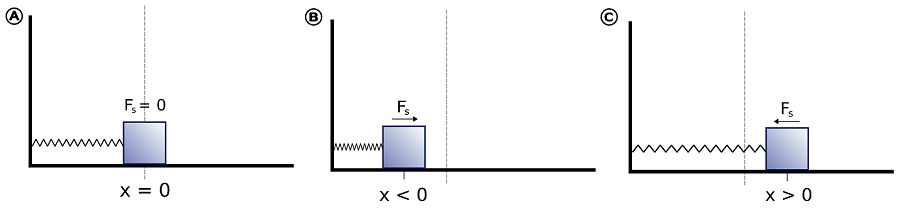
compton — Fig. 59 Illustration of harmonic motion governed by Hook’s law. Any deviation from equilibrium (resting) position is met with restoring force. In the absence of friction the bead keeps oscillating around equilibrium position.#

\[ F=-kx \]

This is Hooke’s law, where minus sign indicates that the direction of force is always towards restoring equilibrium location.
The constant k characterizes stiffness of the spring and is called spring constant.

Solving harmonic oscillator problem#

The classical equation of motion for a one-dimensional simple harmonic oscillator with a particle of mass m attached to a spring having spring constant k generates mechanical waves.

\[m \ddot x=−kx\]

\[m \ddot x+kx = 0 \,\,\,\,\rightarrow \,\,\,\, \ddot{x}+\omega^2 x =0\]

The intorduced constant \(\omega\) will be seen as the frequency oscillations.Note that frequency is inversly porportional to mass (heavier objects with same spring constant oscillate rapdily around equilibrium) and proprotional to spring constant (stiffer springs increase oscillations around equilibrium for same mass)

\[\omega=\Big(\frac{k}{m}\Big)^{1/2}\]

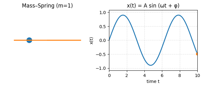
The differneital equation is a simple second order, linear ODE which can be solved by a standard trick of pluggin exponential \(x(t)=e^{\alpha t}\) and convertin the problem to algebraic equation. The solution is

\[ x(t)= A sin(\omega t+\phi) \]

The two constnants are: \(A\) the amplitude of oscillations and \(\phi\) is constant specifying the initial position of the bead.

---------------------------------------------------------------------------
KeyboardInterrupt                         Traceback (most recent call last)
Cell In[1], line 53
     51 # Inline display in Jupyter / Jupyter Book
     52 plt.close()  # Prevents static display of the last frame
---> 53 HTML(anim1.to_jshtml() + "<br><hr><br>" + anim2.to_jshtml())

File /opt/hostedtoolcache/Python/3.8.18/x64/lib/python3.8/site-packages/matplotlib/animation.py:1352, in Animation.to_jshtml(self, fps, embed_frames, default_mode)
   1348         path = Path(tmpdir, "temp.html")
   1349         writer = HTMLWriter(fps=fps,
   1350                             embed_frames=embed_frames,
   1351                             default_mode=default_mode)
-> 1352         self.save(str(path), writer=writer)
   1353         self._html_representation = path.read_text()
   1355 return self._html_representation

File /opt/hostedtoolcache/Python/3.8.18/x64/lib/python3.8/site-packages/matplotlib/animation.py:1103, in Animation.save(self, filename, writer, fps, dpi, codec, bitrate, extra_args, metadata, extra_anim, savefig_kwargs, progress_callback)
   1100 for data in zip(*[a.new_saved_frame_seq() for a in all_anim]):
   1101     for anim, d in zip(all_anim, data):
   1102         # TODO: See if turning off blit is really necessary
-> 1103         anim._draw_next_frame(d, blit=False)
   1104         if progress_callback is not None:
   1105             progress_callback(frame_number, total_frames)

File /opt/hostedtoolcache/Python/3.8.18/x64/lib/python3.8/site-packages/matplotlib/animation.py:1139, in Animation._draw_next_frame(self, framedata, blit)
   1137 self._pre_draw(framedata, blit)
   1138 self._draw_frame(framedata)
-> 1139 self._post_draw(framedata, blit)

File /opt/hostedtoolcache/Python/3.8.18/x64/lib/python3.8/site-packages/matplotlib/animation.py:1164, in Animation._post_draw(self, framedata, blit)
   1162     self._blit_draw(self._drawn_artists)
   1163 else:
-> 1164     self._fig.canvas.draw_idle()

File /opt/hostedtoolcache/Python/3.8.18/x64/lib/python3.8/site-packages/matplotlib/backend_bases.py:2082, in FigureCanvasBase.draw_idle(self, *args, **kwargs)
   2080 if not self._is_idle_drawing:
   2081     with self._idle_draw_cntx():
-> 2082         self.draw(*args, **kwargs)

File /opt/hostedtoolcache/Python/3.8.18/x64/lib/python3.8/site-packages/matplotlib/backends/backend_agg.py:400, in FigureCanvasAgg.draw(self)
    396 # Acquire a lock on the shared font cache.
    397 with RendererAgg.lock, \
    398      (self.toolbar._wait_cursor_for_draw_cm() if self.toolbar
    399       else nullcontext()):
--> 400     self.figure.draw(self.renderer)
    401     # A GUI class may be need to update a window using this draw, so
    402     # don't forget to call the superclass.
    403     super().draw()

File /opt/hostedtoolcache/Python/3.8.18/x64/lib/python3.8/site-packages/matplotlib/artist.py:95, in _finalize_rasterization.<locals>.draw_wrapper(artist, renderer, *args, **kwargs)
     93 @wraps(draw)
     94 def draw_wrapper(artist, renderer, *args, **kwargs):
---> 95     result = draw(artist, renderer, *args, **kwargs)
     96     if renderer._rasterizing:
     97         renderer.stop_rasterizing()

File /opt/hostedtoolcache/Python/3.8.18/x64/lib/python3.8/site-packages/matplotlib/artist.py:72, in allow_rasterization.<locals>.draw_wrapper(artist, renderer)
     69     if artist.get_agg_filter() is not None:
     70         renderer.start_filter()
---> 72     return draw(artist, renderer)
     73 finally:
     74     if artist.get_agg_filter() is not None:

File /opt/hostedtoolcache/Python/3.8.18/x64/lib/python3.8/site-packages/matplotlib/figure.py:3175, in Figure.draw(self, renderer)
   3172         # ValueError can occur when resizing a window.
   3174 self.patch.draw(renderer)
-> 3175 mimage._draw_list_compositing_images(
   3176     renderer, self, artists, self.suppressComposite)
   3178 for sfig in self.subfigs:
   3179     sfig.draw(renderer)

File /opt/hostedtoolcache/Python/3.8.18/x64/lib/python3.8/site-packages/matplotlib/image.py:131, in _draw_list_compositing_images(renderer, parent, artists, suppress_composite)
    129 if not_composite or not has_images:
    130     for a in artists:
--> 131         a.draw(renderer)
    132 else:
    133     # Composite any adjacent images together
    134     image_group = []

File /opt/hostedtoolcache/Python/3.8.18/x64/lib/python3.8/site-packages/matplotlib/artist.py:72, in allow_rasterization.<locals>.draw_wrapper(artist, renderer)
     69     if artist.get_agg_filter() is not None:
     70         renderer.start_filter()
---> 72     return draw(artist, renderer)
     73 finally:
     74     if artist.get_agg_filter() is not None:

File /opt/hostedtoolcache/Python/3.8.18/x64/lib/python3.8/site-packages/matplotlib/axes/_base.py:3064, in _AxesBase.draw(self, renderer)
   3061 if artists_rasterized:
   3062     _draw_rasterized(self.figure, artists_rasterized, renderer)
-> 3064 mimage._draw_list_compositing_images(
   3065     renderer, self, artists, self.figure.suppressComposite)
   3067 renderer.close_group('axes')
   3068 self.stale = False

File /opt/hostedtoolcache/Python/3.8.18/x64/lib/python3.8/site-packages/matplotlib/image.py:131, in _draw_list_compositing_images(renderer, parent, artists, suppress_composite)
    129 if not_composite or not has_images:
    130     for a in artists:
--> 131         a.draw(renderer)
    132 else:
    133     # Composite any adjacent images together
    134     image_group = []

File /opt/hostedtoolcache/Python/3.8.18/x64/lib/python3.8/site-packages/matplotlib/artist.py:72, in allow_rasterization.<locals>.draw_wrapper(artist, renderer)
     69     if artist.get_agg_filter() is not None:
     70         renderer.start_filter()
---> 72     return draw(artist, renderer)
     73 finally:
     74     if artist.get_agg_filter() is not None:

File /opt/hostedtoolcache/Python/3.8.18/x64/lib/python3.8/site-packages/matplotlib/axis.py:1395, in Axis.draw(self, renderer, *args, **kwargs)
   1392     tick.draw(renderer)
   1394 # Shift label away from axes to avoid overlapping ticklabels.
-> 1395 self._update_label_position(renderer)
   1396 self.label.draw(renderer)
   1398 self._update_offset_text_position(tlb1, tlb2)

File /opt/hostedtoolcache/Python/3.8.18/x64/lib/python3.8/site-packages/matplotlib/axis.py:2614, in YAxis._update_label_position(self, renderer)
   2610     return
   2612 # get bounding boxes for this axis and any siblings
   2613 # that have been set by `fig.align_ylabels()`
-> 2614 bboxes, bboxes2 = self._get_tick_boxes_siblings(renderer=renderer)
   2615 x, y = self.label.get_position()
   2616 if self.label_position == 'left':

File /opt/hostedtoolcache/Python/3.8.18/x64/lib/python3.8/site-packages/matplotlib/axis.py:2149, in Axis._get_tick_boxes_siblings(self, renderer)
   2147 axis = getattr(ax, f"{axis_name}axis")
   2148 ticks_to_draw = axis._update_ticks()
-> 2149 tlb, tlb2 = axis._get_ticklabel_bboxes(ticks_to_draw, renderer)
   2150 bboxes.extend(tlb)
   2151 bboxes2.extend(tlb2)

File /opt/hostedtoolcache/Python/3.8.18/x64/lib/python3.8/site-packages/matplotlib/axis.py:1316, in Axis._get_ticklabel_bboxes(self, ticks, renderer)
   1314 if renderer is None:
   1315     renderer = self.figure._get_renderer()
-> 1316 return ([tick.label1.get_window_extent(renderer)
   1317          for tick in ticks if tick.label1.get_visible()],
   1318         [tick.label2.get_window_extent(renderer)
   1319          for tick in ticks if tick.label2.get_visible()])

File /opt/hostedtoolcache/Python/3.8.18/x64/lib/python3.8/site-packages/matplotlib/axis.py:1316, in <listcomp>(.0)
   1314 if renderer is None:
   1315     renderer = self.figure._get_renderer()
-> 1316 return ([tick.label1.get_window_extent(renderer)
   1317          for tick in ticks if tick.label1.get_visible()],
   1318         [tick.label2.get_window_extent(renderer)
   1319          for tick in ticks if tick.label2.get_visible()])

File /opt/hostedtoolcache/Python/3.8.18/x64/lib/python3.8/site-packages/matplotlib/text.py:958, in Text.get_window_extent(self, renderer, dpi)
    953 if self._renderer is None:
    954     raise RuntimeError(
    955         "Cannot get window extent of text w/o renderer. You likely "
    956         "want to call 'figure.draw_without_rendering()' first.")
--> 958 with cbook._setattr_cm(self.figure, dpi=dpi):
    959     bbox, info, descent = self._get_layout(self._renderer)
    960     x, y = self.get_unitless_position()

File /opt/hostedtoolcache/Python/3.8.18/x64/lib/python3.8/contextlib.py:113, in _GeneratorContextManager.__enter__(self)
    111 del self.args, self.kwds, self.func
    112 try:
--> 113     return next(self.gen)
    114 except StopIteration:
    115     raise RuntimeError("generator didn't yield") from None

File /opt/hostedtoolcache/Python/3.8.18/x64/lib/python3.8/site-packages/matplotlib/cbook/__init__.py:2024, in _setattr_cm(obj, **kwargs)
   2021 # if we are dealing with a property (but not a general descriptor)
   2022 # we want to set the original value back.
   2023 if isinstance(cls_orig, property):
-> 2024     origs[attr] = orig
   2025 # otherwise this is _something_ we are going to shadow at
   2026 # the instance dict level from higher up in the MRO.  We
   2027 # are going to assume we can delattr(obj, attr) to clean
   (...)
   2032 # currently have any custom descriptors.
   2033 else:
   2034     origs[attr] = sentinel

KeyboardInterrupt: 

../_images/8a1c099983adf0e983baf93ca188b443247c9cc3971ec1b3031ea5a6504306a9.png

Energy of the harmonic oscillator#

In classical mechanics when we have a conservative system (no frictions, energy conserved) the force is a gradient of a potential energy

\[F = - \frac{\partial V(x)}{\partial x}\]

This means the steeper the potential the higher the force and minus sign indicates that force is restoring system to its equilibrium position.
The potential energy can be obtained by integrating:

\[ V(x)= - \int F dx = - \int (-kx) dx =\frac{kx^2}{2}+C\]

Thus the potential energy for a simple harmonic oscillator is a parabolic function of displacement. It is convenient to set \(C=0\) and measure potential energy relative to equilibrium state \(V(x=0)=0\)
The total energy consisting of kinetic and potential enregies will be used to obtain Schordinger equation.

\[E=\frac{p^2}{2m} + \frac{kx^2}{2}\]

Diatomic molecules and two-body problem#

Diatomic molecule is stable because the same force is acting on both ends

\[\begin{split}m_1\ddot{x_1}=kx \\ m_2\ddot{x_2}=-kx\end{split}\]

By expressing equations of motion in terms of the center of mass which, we find that center of mass moves freely without acceleration.

\[m_1\ddot{x_1}+ m_2\ddot{x_2}=0\,\,\,\, \rightarrow \frac{m_1\ddot{x_1}+ m_2\ddot{x_2}}{m_1+m_2}=\ddot{x}_{com}=0\]

Next by taking difference between coordinates \(\ddot{x_2}=-\frac{k}{m_2}x_2\) and \(\ddot{x_1}=\frac{k}{m_1}x_1\)we expres the equations of motion in terms of relative distance

\[\ddot{x}=\ddot{x_2} - \ddot{x_1} =-\Big(\frac{1}{m_1}+\frac{1}{m_2} \Big)kx=-\frac{k}{\mu}x\]

This equation looks identical to the probem of bead anchored to wall with a spring. We have thus managed to reduce the two body probelm to a one modey problem by replacing masses of bodies with a reduced mass: \(\mu=\frac{1}{m_1}+\frac{1}{m_2}=\frac{m_1 m_2}{m_1+m_2}\)

### Beads and springs model of molecules

- Before discussing the harmonic oscillator approximation let us reflect on when this would be a good approximation and uner which cirumstances it will break down? For an aribtarry potential energy funciton of x we can carry out Taylor's expansion around equilibrium bond length $x_0$ obtaining infinitey series. 

$$U(x) = U(x_0)+U'(x_0)(x-x_0)+\frac{1}{2!}U''(x_0)(x-x_0)^2+\frac{1}{3!}U'''(x_0)(x-x_0)^3+...$$

:::{figure-md} markdown-fig

<img src="images/harm_approx.png" alt="harmls" class="bg-primary mb-1" width="300px">

Deviation from simple harmonic potential approximation (red curve) of true/exact potential (blue curve) with cubic term (green)

Setting energy scale to be relative to \(U(x_0)=0\) and recongizing that first derivative vanishes at minima \(x_0\) we have

\[U(x) = \frac{1}{2!}k(x-x_0)^2+\frac{1}{3!}\gamma(x-x_0)^3+...\]

Hence we see that the Harmonic approximation is only the first non vanishing term! Furthermore we see that spring constant k and subsequent anharmonicity consnats such as \(\gamma\) are higher order derivatives of potential energy. That is the more non-linear the potential the higer the contribution of these terms. And vice verse clsoer the potential to quadratic form the more accurate is the harmonic assumtion.