
What you will learn
A wave is a self-propagating disturbance that transfers energy, momentum, and information through a medium, without transporting matter.
The behavior of waves is governed by the wave equation, a partial differential equation (PDE) that describes their spatial and temporal evolution.
Two major classes of waves we will be examining are Standing waves which remain fixed in space, exhibiting nodes and antinodes.
Traveling waves which propagate through space, transferring energy from one location to another.
Types of Waves#
Disturbance of medium Sound Waves. Waves on a guitar string. Waves propogating on the surface of the water
Quantum mechanical waves They will be described by complex wavefunctions providing us expanation for the wave like behavior electrons and atoms.
Electromagnetic waves (e.g. light, UV, X-rays) this is the only kind of wave which does not require a medium! EM waves can travel in vacuum. In a sense, an EM wave “rolls out its own carpet” hence creating its own medium as it moves forward.
Gravitational waves traveling through spacetime!
Fig. 34 Visualiziing 1D propagating (or traveling) and standing waves waves. Traveling waves move with respect to a fixed reference frame. Standing waves move in place.#
Fig. 35 Transverse waves carry distrubance perpendicular to the direction of wave propogation. Longitudinal waves carry disturbance along the direction of wave propogation.#
Defining wave mathematically#
Since wave is a moving disturbance \(u\), we describe this disturbance (e.g. vertical displacement) by specifying change of disturbance as a function of space \(x\) and time \(t\) via some mathematical function \(f\):
Imagine surfing on an ocean wave. For an observer (surfer) standing on a wave the wave stands still at the same coordinate \(x'\).
For the observer standing on the shore the coordinate x of wave front moves away with a constant velocity:
Assuming that shape of the wave stays the same we can express the motion of wave in the reference frame of the still observer:
To see why \(f(x-vt)\) implies motion to the right take a constant front of the wave \(x-vt=const\) which shows that \(x = vt +const\) and vice versa for \(f(x+vt)\)
Show code cell source
import numpy as np
import matplotlib.pyplot as plt
from matplotlib.animation import FuncAnimation
from IPython.display import HTML, display
# Wave shape (Gaussian)
def f(x):
return np.exp(-x**2)
# Parameters
v = 1.0
x = np.linspace(-10, 10, 600)
t_step = 0.08
n_frames = 150
# Figure
fig, ax = plt.subplots(figsize=(6, 4))
(line_right,) = ax.plot([], [], lw=2, label=r"$f(x-vt)$ (right)")
(line_left,) = ax.plot([], [], lw=2, ls="--", label=r"$f(x+vt)$ (left)")
ax.set_xlim(-10, 10)
ax.set_ylim(-0.1, 1.1)
ax.set_xlabel("x")
ax.set_ylabel("u(x,t)")
ax.legend(loc="upper right")
ax.set_title("Traveling waves: $f(x\mp vt)$")
def init():
line_right.set_data([], [])
line_left.set_data([], [])
return line_right, line_left
def update(frame):
t = frame * t_step
line_right.set_data(x, f(x - v*t)) # right-moving
line_left.set_data(x, f(x + v*t)) # left-moving
return line_right, line_left
ani = FuncAnimation(fig, update, frames=n_frames, init_func=init, blit=True, interval=40)
# >>> Display as inline HTML (no saving needed)
display(HTML(ani.to_jshtml()))
plt.close(fig)
Periodic traveling waves.#
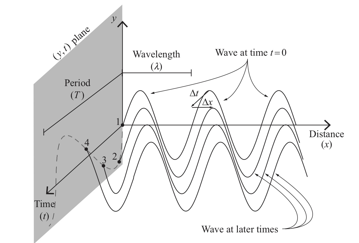
Fig. 36 Wave that is periodic in space and time#
We will be working a lot with periodic waves that have a periodic shape hence can be described by sine or cosine or their combination. Here is a general expression of sin wave:
Let us now turn this sinusoidal form into a wave traveling along x axis:
Amplitude \(A\): specifies maximum disturbance.
Wave number \(k\): specifies periodicity in space.
Angular frequency \(\omega=kv\): specifies periodicity in time.
Initial phase \(\phi\): initial phase. E.g where does wave start at \(t=0\) \(x=0\) often we just set \(\phi=0\).
When describing waves it is much more convenient to work with complex representation. One can always extract real or imaginary part after calculations.
Complex exponential representation of waves
We can visualize sin and cos components on complex exponential and also visualize the phasor which is the change of exponential driven by chaneg of \(t\) for any fixed value \(x\).
Show code cell source
import numpy as np
import matplotlib.pyplot as plt
from matplotlib.animation import FuncAnimation
from IPython.display import HTML, display
# -----------------------
# Parameters
# -----------------------
k = 2 * np.pi / 5.0 # wavenumber
omega = 2 * np.pi / 3.0 # angular frequency
x = np.linspace(-10, 10, 600)
x0 = 0.0 # fixed position for phasor
t_step = 0.08
n_frames = 140 # keep size reasonable for inline JS
# -----------------------
# Figure with two subplots
# -----------------------
fig, (ax_wave, ax_phasor) = plt.subplots(1, 2, figsize=(10, 4))
# Left subplot: real and imaginary parts
(line_real,) = ax_wave.plot([], [], lw=2, label="Re$\\{e^{i(kx-\\omega t)}\\}$")
(line_imag,) = ax_wave.plot([], [], lw=2, ls="--", label="Im$\\{e^{i(kx-\\omega t)}\\}$")
ax_wave.set_xlim(x.min(), x.max())
ax_wave.set_ylim(-1.2, 1.2)
ax_wave.set_xlabel("x")
ax_wave.set_ylabel("Amplitude")
ax_wave.set_title("Real and Imaginary Parts vs x")
ax_wave.legend(loc="upper right")
# Right subplot: phasor
theta = np.linspace(0, 2*np.pi, 400)
ax_phasor.plot(np.cos(theta), np.sin(theta), lw=1) # unit circle
(point_line,) = ax_phasor.plot([], [], lw=2) # line from origin to tip
(point_tip,) = ax_phasor.plot([], [], marker='o', lw=0)
ax_phasor.set_aspect('equal', 'box')
ax_phasor.set_xlim(-1.2, 1.2)
ax_phasor.set_ylim(-1.2, 1.2)
ax_phasor.set_xlabel("Re")
ax_phasor.set_ylabel("Im")
ax_phasor.set_title(f"Phasor at x0 = {x0}")
def init():
line_real.set_data([], [])
line_imag.set_data([], [])
point_line.set_data([], [])
point_tip.set_data([], [])
return (line_real, line_imag, point_line, point_tip)
def update(frame):
t = frame * t_step
phase = k * x - omega * t
# Left subplot updates
line_real.set_data(x, np.cos(phase))
line_imag.set_data(x, np.sin(phase))
# Right subplot updates (phasor at x0)
angle = k * x0 - omega * t
z = np.cos(angle) + 1j*np.sin(angle)
point_line.set_data([0, z.real], [0, z.imag])
point_tip.set_data([z.real], [z.imag])
return (line_real, line_imag, point_line, point_tip)
ani = FuncAnimation(fig, update, frames=n_frames, init_func=init, blit=True, interval=40)
# Display as inline HTML JS animation; then close to avoid duplicate static rendering
display(HTML(ani.to_jshtml()))
plt.close(fig)